Using R to Animate the Population Density of Ghana
Introduction
It has been a while since I wrote a blog for this website. This is mostly due to the fact that I do no longer have to work from home and because worked has really picked up again since Ghana lifted its travel restrictions and I could go back to work in person. Also, the code for this blog took me some real head-scratching and I probably discarded close to 20.000 lines of code along the way. So this blog is a lot of code and relatively little text. If I find the energy I might come back to it and add some more text, but for now, I will let the images tell the story.
Back to the origin. Browsing through Twitter I came across these pretty cool (albeit not very useful) 3D representations of population density in different places and I wondered if I could just do the same for Ghana (see
here,
here, and
here for examples of what I mean). In this tutorial, I will show to make 3d population density maps and animations using the rayshader package and how to create an insightful leaflet map from raster data.
Packages
These are the packages I use for this blog. I realize there are a lot this time.
library(raster)       # to work with raster data
library(sf)           # to work with shape files
library(viridis)      # for the colour scheme
library(cartography)  # to help with the plotting of the maps
library(tanaka)       # to make the Tanaka plots
library(rworldmap)    # to get the shape file of Ghana
library(tidyverse)    # to do the data wrangling
library(tmap)         # to make the static 2d maps
library(SpatialPosition) # to calculate some spatial statistics
library(leaflet)      # to make the interactive versions of the map
library(rayshader)    # to make the 3D plot
library(rayrender)    # to to render the 3D plot
library(tweenr)       # to interpolate data
library(stringr)      # to work with text data
library(scales)       # to create nice scales in the legend
library(lubridate)    # to work with dates
library(gdata)        # to delete objects from the environment
library(zoo)          # to interpolate data
library(showtext)     # to add fonts
Download the Population Data
There are many different sources of population data available online. Some are based on countries censuses, some on satellite data, and some on a combination of these two. Most of these population density files will be in a raster format file (usually a GeoTIFF) and have a certain resolution (e.g. 1km, 250m or 100m). The more precise the resolution, the more granular the data (and the larger the data file). For this blog, I will use the one file with an accuracy of 100m from AfriPop, with as the unit of measurement the “Estimated persons per grid square” (for more information and to download the data see: https://www.worldpop.org/doi/10.5258/SOTON/WP00098). I also will use a file with an accuracy of 1 km x 1 km Grid provided by the European Commission Science Hub, called the Global Human Settlement Layer (GHSL) and specifically the GHS-POP dataset (“This spatial raster dataset depicts the distribution of population, expressed as the number of people per cell."). More information on that dataset can be found
here. Both these datasets use 2015 as the reference year.
Let start with simply plotting the population density in Ghana in 2015. Due to the nature of population density estimates using a continuous colour scale is not very useful and is it probably better to use some type of binning. I am using the kmeans clustering algorithm to create the 18 bins. Since this algorithm uses a random starting point, it yields slightly different results every time. That is why a set a seed to guarantee reproducibility of the plot.
# load the raster data
pop_density_Ghana    <- raster(x = "GHA15adj_040213.tif")

# set colour breaks
cols <- c("#F7E1C6", "#EED4C1", "#E5C9BE", "#DCBEBA", "#D3B3B6", "#CAA8B3",
          "#C19CAF", "#B790AB", "#AC81A7", "#A073A1", "#95639D", "#885497",
          "#7C4692", "#6B3D86", "#573775", "#433266", "#2F2C56", "#1B2847")

set.seed(5)
tm_shape(pop_density_Ghana,
           raster.downsample = FALSE) +
  tm_raster(
    style = "kmeans",
    title = "Number of people\nper 10.000m2",
    n     = 18,
    palette = cols,
    legend.hist = FALSE
  ) +
  tm_legend(outside = TRUE) +
  tm_layout(fontface = 6,
            compass.type = "arrow") +
  tm_compass()

It is clear that the south of Ghana is much more densely populated than the North and that two highly densely populated urban areas that stand out (Accra and Kumasi). A 100m x 100m grid is really quite a high resolution and does allow me to zoom in. One of the nice things of working with raster data in R is that you can subset certain areas using a shapefile. So using a shapefile of the different neighbourhoods of Accra, let us zoom in to Accra.
# Read Accra file
Accra_Neigborhoods   <- st_read("AccraFMVs2010.shp", quiet = TRUE)
# combine the different neighbourhoods into one shapefile
Accra_outline        <- st_union(Accra_Neigborhoods)
# Set the projection to be equal to the population density raster file
Accra_outline_lonlat <- st_transform(Accra_outline, crs = crs(pop_density_Ghana))
### crop out just Accra
popdens_Accra        <- crop(pop_density_Ghana, extent(as_Spatial(Accra_outline_lonlat)))
popdens_Accra        <- mask(popdens_Accra, as_Spatial(Accra_outline_lonlat))

### crop out just Accra
popdens_Accra <- crop(pop_density_Ghana, extent(as_Spatial(Accra_outline_lonlat)))
popdens_Accra <- mask(popdens_Accra, as_Spatial(Accra_outline_lonlat))

# set seed
set.seed(1)
# plot density of Accra
tm_shape(popdens_Accra,
           raster.downsample = FALSE) +
  tm_raster(style       = "kmeans",
            n           = 18,
            title       = "Number of people\nper 10.000m2",
            palette     = cols,
            legend.hist = FALSE) +
  tm_legend(outside  = TRUE)  +
  ## add the boundaries of the neighborhoods
  tm_shape(Accra_Neigborhoods) +
  tm_borders(lwd = .5,
             lty = "solid" ,
             col = "black") +
  tm_layout(fontface     = 6,
            compass.type = "arrow") +
  tm_compass()

Again, we can clearly see that there are large differences in the population density of different neighbourhoods in Accra.
One of the convenient things about raster data is the fact that it in essence is just a matrix. This means that all you can do all the mathematical arithmetics you can do on a matrix, such as taking means, summing and multiplying, on raster data easily. So for example, if you want to compare the population in Ghana in 1975 to that in 2015 and see where in Ghana, relatively, there has been the highest population growth. You can simply for every cell use calculate $\frac{pop_{2015}- pop_{1975}}{pop_{1975}}\cdot100%$. Or you could calculate for every cell what percentage of the population lives in that cell (in total Ghana exists of 3,829,204 different cells in the data I will be using, so al those percentage would be tiny). Speaking of the data I will be using, for this plot, I am using the 250m x 250m gridded GHS-POP dataset from the EU for both 1975 and 2015. Unfortunately, this data does not have the nice cut out of Lake volta included and I can’t really be bothered to do that myself. Also, unfortunately, this dataset can either be downloaded for the whole planet (R.I.P. my internet) or in different smaller chunks and Ghana just falls in 4 different of these squares. That is why I downloaded the 8 different chunks (4 for 1975 and 4 for 2015) and combined them myself using the melt function in do.call.
# load all the raster data
pop_250_m_tile_1_2015 <- raster(x = "GHS_POP_E2015_GLOBE_R2019A_54009_250_V1_0_17_7.tif")
pop_250_m_tile_2_2015 <- raster(x = "GHS_POP_E2015_GLOBE_R2019A_54009_250_V1_0_17_8.tif")
pop_250_m_tile_3_2015 <- raster(x = "GHS_POP_E2015_GLOBE_R2019A_54009_250_V1_0_18_7.tif")
pop_250_m_tile_4_2015 <- raster(x = "GHS_POP_E2015_GLOBE_R2019A_54009_250_V1_0_18_8.tif")

# merge the 4 different cells
list_tiles_2015       <- list(pop_250_m_tile_1_2015,
                              pop_250_m_tile_2_2015,
                              pop_250_m_tile_3_2015,
                              pop_250_m_tile_4_2015)

West_africa_pop_2015  <- do.call(merge, list_tiles_2015)

# same for 1975
pop_250_m_tile_1_1975 <- raster(x = "GHS_POP_E1975_GLOBE_R2019A_54009_250_V1_0_17_7.tif")
pop_250_m_tile_2_1975 <- raster(x = "GHS_POP_E1975_GLOBE_R2019A_54009_250_V1_0_17_8.tif")
pop_250_m_tile_3_1975 <- raster(x = "GHS_POP_E1975_GLOBE_R2019A_54009_250_V1_0_18_7.tif")
pop_250_m_tile_4_1975 <- raster(x = "GHS_POP_E1975_GLOBE_R2019A_54009_250_V1_0_18_8.tif")

list_tiles_1975      <- list(pop_250_m_tile_1_1975,
                             pop_250_m_tile_2_1975,
                             pop_250_m_tile_3_1975,
                             pop_250_m_tile_4_1975)

West_africa_pop_1975 <- do.call(merge, list_tiles_1975)


# load a world map to crop  out just Ghana
World_map     <- getMap(resolution = "low")
World_map     <- st_as_sf(World_map)
Ghana_map     <- filter(World_map,  NAME == "Ghana")

# crop it all to the shape of Ghana
Ghana_pop_250m_1975 <-
  crop(West_africa_pop_1975, extent(as_Spatial(st_transform(
    Ghana_map, crs = crs(West_africa_pop_1975)
  ))))
Ghana_pop_250m_1975 <-
  mask(Ghana_pop_250m_1975, as_Spatial(st_transform(Ghana_map, crs = crs(
    West_africa_pop_1975
  ))))

Ghana_pop_250m_2015 <-
  crop(West_africa_pop_2015, extent(as_Spatial(st_transform(
    Ghana_map, crs = crs(West_africa_pop_2015)
  ))))
Ghana_pop_250m_2015 <-
  mask(Ghana_pop_250m_2015, as_Spatial(st_transform(Ghana_map, crs = crs(
    West_africa_pop_2015
  ))))
As the value of each cell indicates the number of people in that cell, the sum of all cells should make up the total population. This is easy to check
sum(as.matrix(Ghana_pop_250m_1975$layer), na.rm = T)
## [1] 9683598
sum(as.matrix(Ghana_pop_250m_2015$layer), na.rm = T)
## [1] 26877258
In 1975 Ghana’s population was 9,683,598 and in 2015 26,877,258. Now we can plot the population of Ghana in 1975, 2015, absolute change, relative change, the share of population per cell for both and 1975 and 2015 and the change in these values. Instead of making 7 different plots, I decided to just make one interactive leaflet application and add the 7 plots as different layers. Thankfully tmap and leaflet play nicely with each other, so that is quite a straightforward task. I just make tmap figure with all the different plots and then use the tmap_leaflet() function to transform it into a single leaflet application.
# calculate stats

Ghana_pop_250m_percent_increase <- (Ghana_pop_250m_2015 - Ghana_pop_250m_1975)/ Ghana_pop_250m_1975 * 100
Ghana_pop_250m_percent_increase[Ghana_pop_250m_percent_increase < -1000000] <- -100
Ghana_pop_250m_percent_increase[Ghana_pop_250m_percent_increase > 1000000] <- 1000
Ghana_pop_250m_percent_increase[is.na(Ghana_pop_250m_percent_increase)] <- 0
Ghana_pop_250m_percent_increase <- mask(Ghana_pop_250m_percent_increase,
                                        as_Spatial(st_transform(Ghana_map, crs = crs(West_africa_pop_2015))))

diff_population      <- West_africa_pop_2015- West_africa_pop_1975
popdens_change_Ghana <- crop(diff_population,
                             extent(as_Spatial(st_transform(Ghana_map, crs = crs(diff_population)))))
popdens_change_Ghana <- mask(popdens_change_Ghana,
                             as_Spatial(st_transform(Ghana_map, crs = crs(diff_population))))

Ghana_pop_250m_1975_trans  <- projectRaster(from = Ghana_pop_250m_1975,
                                            crs = crs(Accra_Neigborhoods))
Ghana_pop_250m_2015_trans  <- projectRaster(from = Ghana_pop_250m_2015,
                                            crs = crs(Accra_Neigborhoods))
popdens_change_Ghana_trans <- projectRaster(from = popdens_change_Ghana,
                                            crs = crs(Accra_Neigborhoods))
Ghana_pop_250m_percent_increase_trans <- projectRaster(from = Ghana_pop_250m_percent_increase,
                                                       crs = crs(Accra_Neigborhoods))
Ghana_pop_250m_1975_rel <- Ghana_pop_250m_1975/sum(as.matrix(Ghana_pop_250m_1975$layer), na.rm = T) * 100
Ghana_pop_250m_2015_rel <- Ghana_pop_250m_2015/sum(as.matrix(Ghana_pop_250m_2015$layer), na.rm = T) * 100
diff_relative <- Ghana_pop_250m_2015_rel - Ghana_pop_250m_1975_rel

Ghana_pop_250m_1975_rel_trans <- projectRaster(from = Ghana_pop_250m_1975_rel,
                                               crs = crs(Accra_Neigborhoods))
Ghana_pop_250m_2015_rel_trans <- projectRaster(from = Ghana_pop_250m_2015_rel,
                                               crs = crs(Accra_Neigborhoods))
diff_relative_trans <- projectRaster(from = diff_relative, crs = crs(Accra_Neigborhoods))


bks_4 <- c(0,1, 5, 10, 15,  25,
           50, 75, 100,
           150, 200, 250, 500,750,
           1000, 2000, 5000, 10000, 300000)

bks_5 <- c(0, 0.00001, 0.000025, 0.00005,0.000075,
           0.0001, 0.00025, 0.0005, 0.00075 , 0.001,
           0.0025, 0.005 , 0.0075, 0.01, 0.025,
           0.05, 0.075, 0.1, 0.25, 0.5)


# creat my own labelling function
My_label <- function(x, final = "+", lower = F, lower_string = "< ", suffix_log = F, suffix = "%"){
  if(suffix_log){
    x <- paste0(format(x, big.mark = ",",drop0trailing = T, scientific= F, trim = T),suffix )
  }
  label_p <- c()
  if(lower == F){
  for(i in 1:(length(x)-2)){
    label_p[i] <- paste0(format(x[i], big.mark = ",",drop0trailing = T, scientific= F, trim = T),
                         " to ",
                         format(x[i +1], big.mark = ",",drop0trailing = T, scientific= F, trim = T ))
  }
  labels <- c(label_p, paste0(format(x[length(x)-1],big.mark = ",",drop0trailing = T, scientific= F, trim = T ) , final))
  }else{
    for(i in 2:(length(x)-2)){
      label_p[i] <- paste0(format(x[i], big.mark = ",",drop0trailing = T, scientific= F, trim = T),
                           " to ",
                           format(x[i +1], big.mark = ",",drop0trailing = T, scientific= F, trim = T))
    }
    labels <- c(paste0(lower_string, format(x[2],
                                  big.mark = ","
                                  ,drop0trailing = T,
                                  scientific= F,
                                  trim = T)),
      na.omit(label_p),
      paste0(format(x[length(x)-1],
                    big.mark = ",",
                    drop0trailing = T,
                    scientific= F, trim = T ) ,
             final))
  }


  labels[labels == "-0.00001% to 0.00001%"] <- "no change"
  labels[labels == "-0.00001 to 0.00001"]   <- "no change"

  labels
}


# add all the layers together
combined_maps <- tm_shape(Ghana_pop_250m_1975_trans,
                        raster.downsample = F) +
  tm_raster(title = "1975 n people<br>in 250m x 250m",
            group = "Ghana population 1975",
            breaks = bks_4,
            alpha = .7,
             labels = My_label(bks_4),
            palette = cols,
            legend.hist = F) +
  tm_shape(Ghana_pop_250m_2015_trans,
           raster.downsample = F) +
  tm_raster(title = "2015 n people<br>in 250m x 250m",
            group = "Ghana population 2015",
            breaks = bks_4,
            alpha = .7,
            labels = My_label(bks_4),
            palette = cols,
            legend.hist = F) +
  tm_shape(popdens_change_Ghana_trans,
           raster.downsample = F) +
  tm_raster(title = "difference in n<br> people per square<br>1975 to 2015",
            group = "absolute difference 1975 to 2015",
            midpoint = NA,
            alpha = .7,
            breaks = c(-20000, 0, 5, 10, 50, 75, 100, 200, 250, 500,
                       750, 1000, 2000, 2500,5000, 10000, 15000),
            labels = My_label(c(-20000, 0, 5, 10, 50, 75, 100, 200, 250, 500,
                               750, 1000, 2000, 2500,5000, 10000, 15000),
                             lower = T),
            palette = c("#17521D" ,rev(carto.pal(pal1 = "harmo.pal" ,n1 = 16))),
            legend.hist = F) +
  tm_shape(Ghana_pop_250m_percent_increase_trans,
           raster.downsample = F) +
  tm_raster(title = "percentage change",
            group = "relative change 1975 to 2015",
            midpoint = NA,
            alpha = .7,
            breaks = c(-1000, -10, -5, -1, -0.00001,0.00001,1, 2, 5, 10,20,
                       30, 40, 50, 75,  100, 200, 500, 1000, 1000000),
             labels=My_label(c(-1000, -10, -5, -1, -0.00001,0.00001,1, 2, 5, 10,20,
                                30, 40, 50, 75,  100, 200, 500, 1000, 1000000),
                              lower = T,
                             suffix_log = T),
            palette = c(rev(carto.pal(pal1 = "blue.pal", n1 = 4)),
                        "grey96",
                        carto.pal(pal1 = "red.pal", n1 = 14)),
            legend.hist = F)+
  tm_shape(Ghana_pop_250m_1975_rel_trans,
           raster.downsample = F) +
  tm_raster(title = "% share of<br>total population 1975",
            group = "share of total population per square 1975",
            labels = My_label(bks_5),
            breaks = bks_5,
            alpha = .7,
            palette = c("#B1D2A4",
                        carto.pal(pal1 = "red.pal", n1 = 19)),
            legend.hist = F) +
  tm_shape(Ghana_pop_250m_2015_rel_trans,
                         raster.downsample = F) +
  tm_raster(title = "% share of<br>total population 2015",
            group = "share of total population per square 2015",
            breaks = bks_5,
            alpha = .7,
            labels = My_label(bks_5),
            palette = c("#B1D2A4", carto.pal(pal1 = "red.pal", n1 = 19)),
            legend.hist = F) +
  tm_shape(diff_relative_trans,
           raster.downsample = F) +
  tm_raster(title = "change in share of pop",
            group = "change in share of popopulation",
            alpha = .7,
            labels = My_label(c(-1,-0.1, -0.05,-0.00001,0.00001,0.000025, 0.00005,0.000075, 0.0001,
                                0.00025, 0.0005, 0.00075 , 0.001, 0.0025, 0.005 , 0.0075, 0.01, 1)),
            breaks = c(-1,-0.1, -0.05,-0.00001,0.00001,0.000025, 0.00005,0.000075, 0.0001,
                       0.00025, 0.0005, 0.00075 , 0.001, 0.0025, 0.005 , 0.0075, 0.01, 1),
            palette =  c(rev(carto.pal(pal1 = "blue.pal", n1 = 3)), "grey96",
                         carto.pal(pal1 = "red.pal", n1 = 13)),
            legend.hist = F)


leaflet_map <- tmap_leaflet(combined_maps) %>%
  hideGroup(c("Ghana population 1975",
              "Ghana population 2015",
              "absolute difference 1975 to 2015",
              "relative change 1975 to 2015",
              "share of total population per square 1975",
              "share of total population per square 2015",
              "change in share of popopulation"))

leaflet_map
# htmlwidgets::saveWidget(leaflet_map, "leaflet_map.html")
Three things that stood out to me as interesting:
- around lake Volta between 1975 and 2015 there is clear population growth and many small communities popped up (click on
absolute difference 1975 to 2015layer in the top left corner) - The same is true for the population around new road networks that were built in those 40 years, especially the Cape Coast to Kumasi road is a clear example of that.
- Most cities saw relative population growth between 1975 and 2015, the exception to that seems to be Tamale (in the northeast of the country. Toggle the layer
absolute difference 1975 to 2015to see this In 1975 a larger share of the population lived in Tamale, then did in 2015.
Ok that was fun, but now to the real fun part of making some 3D plots
Make a Tanaka plot
Like I said in the introduction, I would like to create a three-dimensional representation of population density in Ghana. A first way to do so, is a so-called
Tanaka plot.
This is quite easy to do using the SpatialPosition and tanaka packages. This is of course not a real 3D representation, but with the right parameters for the shadow, it is quite close. The GHS_POP_E2015_GLOBE_R2019A_54009_1K_V1_0.tif is the population file for the whole planet, so I need to first crop this to only be limited to only Ghana
# Load raster data
pop2015_1km   <- raster("GHS_POP_E2015_GLOBE_R2019A_54009_1K_V1_0.tif")
Ghana_map     <- st_transform(Ghana_map, crs =  st_crs(pop2015_1km))

# crop out Ghana
pop_1km_Ghana <- crop(pop2015_1km, st_bbox(st_buffer(Ghana_map, .4))[c(1,3,2,4)])

# use the SpatialPosition package to create the smoothed input for the Tanaka plot
Weights_matrix               <- focalWeight(x = pop_1km_Ghana, d= 10000, type = "Gauss")
pop_1km_Ghana_smoothed       <- focal(x = pop_1km_Ghana, w = Weights_matrix, fun = sum, pad = TRUE, padValue = 30)

# reproject this raster data into the correct projection for a map of Ghana
# if you do not do this, you get the default projection which distorts Ghana considerably
pop_1km_Ghana_smoothed_trans <- projectRaster(from = pop_1km_Ghana_smoothed, crs = crs(Accra_Neigborhoods))

# plot the Tanaka plot
bks_2 <- c(0, 10, 25, 50, 75, 100, 150, 200, 250, 300, 400, 500, 600, 700, 750, 1500, 2500, 3000)


# add a font to the plot
font_add_google("Righteous")
showtext_auto()
par(family = "Righteous", mar = c(0, 0, 1.2, 0))

tanaka(x = pop_1km_Ghana_smoothed_trans,
       breaks = bks_2,
       mask = st_transform(Ghana_map, crs = crs(pop_1km_Ghana_smoothed_trans)),
       col = cols,
       legend.pos = "topleft",
       legend.title = "Population Density")
layoutLayer(title = "Smoothed Population Ghana",
            scale = F, frame = F, tabtitle = FALSE)
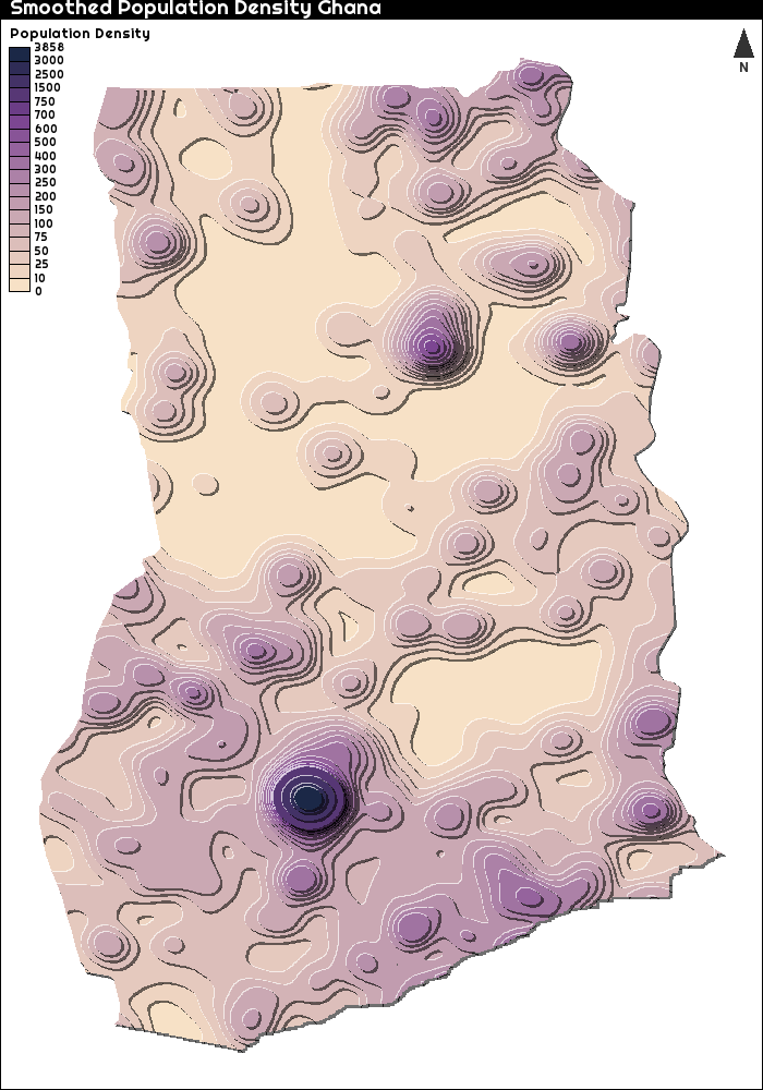
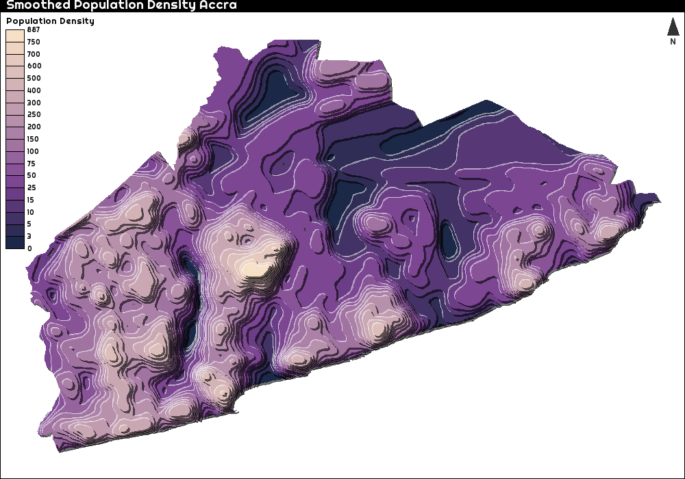
In this plot, we see that the population density in Kumasi (the big hump) seems to be quite a bit higher than in Accra. I can easily make a similar plot for just Accra (to confuse everyone and to spice things up a bit, I reversed the colour scale)
# Need to crop around Accra a bit wider, to make sure the population on the border is actually translated into height
# That is what I use st_buffer
popdens_Accra_2 <- crop(pop_density_Ghana, extent(as_Spatial(st_buffer(Accra_outline_lonlat, 0.04))))
popdens_Accra_2 <- mask(popdens_Accra_2, as_Spatial(st_buffer(Accra_outline_lonlat, 0.04)))

popdens_Accra_2[is.na(popdens_Accra_2$GHA15adj_040213)] <- 0
popdens_Accra_trans <- projectRaster(from = popdens_Accra_2, crs = crs(Accra_Neigborhoods))
Weights_matrix_2        <- focalWeight(x = popdens_Accra_trans, d= 200, type = "Gauss")
popdens_Accra_smoothed  <- focal(x = popdens_Accra_trans, w = Weights_matrix_2, fun = sum, pad = F)

bks_3 <- c(0,3, 5, 10, 15,  25, 50, 75, 100, 150, 200, 250, 300, 400, 500, 600, 700, 750)
par(family="", mar = c(0,0,1.2,0))


font_add_google("Righteous")

showtext_auto()

par(family="Righteous", mar = c(0,0,1.2,0))

tanaka(x = popdens_Accra_smoothed,
       breaks = bks_3,
       col = rev(cols),
       mask = st_transform(Accra_outline, crs = crs(popdens_Accra_smoothed)),
       legend.pos = "topleft",
       legend.title = "Population Density")
layoutLayer(title = "Smoothed Population Accra",
            scale = F,
            frame = T,
            north = T,
            tabtitle = FALSE)
Make a 3D plot using Rayshader
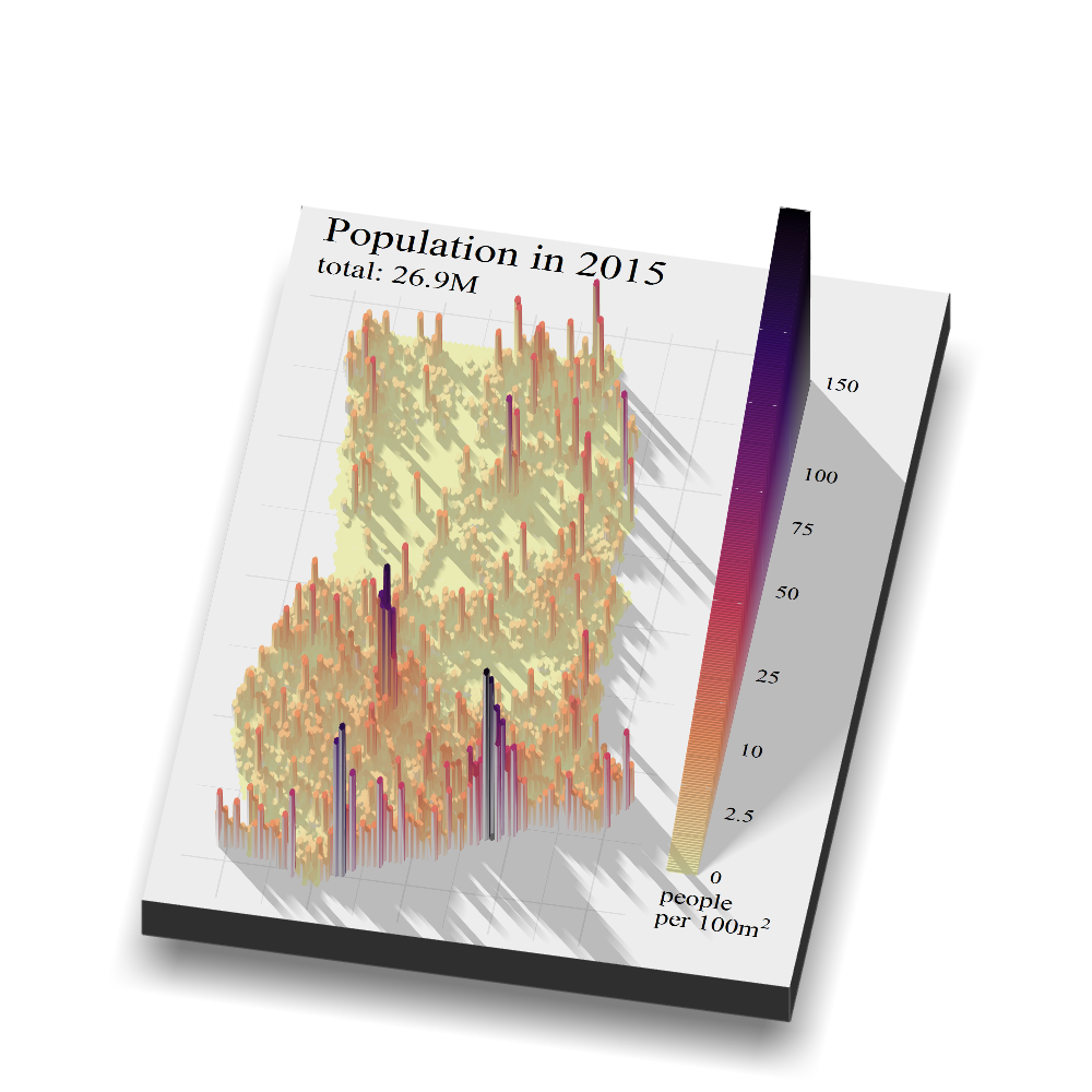
Now, to the actual 3D stuff. Using the great rayshader package it is possible to render most ggplot figures and maps as 3-dimensional objects, including realistic lighting and shadows. To make a plot like this, I first made a normal ggplot hexbin map. A hexbin plot summarizes (by default by taking a mean) for a variable in a 2-dimensional space (the 1d dimensional equivalent would be a histogram or density plot). Because of the high resolution of the raster data, the data is clearer to interpret once it is summarized in these hexagons, as opposed to plotting the raw directly (there are over 3 million data point). To go from raster format data to data that can be summarized in hexagons, I used the rasterToPoints() function. This function transforms the raster data, pixel by pixel, into a dataset with 3 columns (x, y, and whatever the value was of a certain raster pixel). This dataset is then fed into stat_summary_hex() in ggplot. All the other commands are fairly standard ggplot functions and commands. I used a square root transformation of the data (trans = 'sqrt') to give some more weight to a lower value. Without such a transformation, Accra and Kumasi stand out even more as they already do.
To transform this 2 two-dimensional map into a 3D map I use the plot_gg() function from the rayshader package. In this function, you need to set the viewing angle (phi and theta) and the angle and direction from which you want the light to appear (sun angle and angle breaks). This opens a new window with a 3D rendered map. To save a snapshot of this map use render_snapshot().
points_Ghana <- tibble::as_tibble(raster::rasterToPoints(Ghana_pop_250m_2015)) %>%
  mutate(layer  = ifelse(layer  < 0, NA, layer ))

plot_hex_2015 <- points_Ghana  %>%
  ggplot(aes(x = x, y = y, z = layer/(250^2/100^2))) + # the data comes in 250m*250m tiles so we recalculate that to 100m2
  stat_summary_hex(bins = 70, size = 0.5) +
  scale_fill_viridis_c(option = "magma",
                       trans = 'sqrt',
                       direction = -1,
                       limits = c(0, 150),
                       breaks = c(0,2.5, 10, 25, 50, 75, 100, 150),
                       labels = c("0", "2.5","10", "25",  "50",'75', "100", "150" )) +
  theme_minimal()+
  coord_quickmap()+
  labs(x = NULL,
       y = NULL,
       fill = expression(paste("people\nper 100",m^2), sep = ""),
       title = "Population in 2015",
       subtitle =  paste0("total: ", label_number_si(accuracy=0.1)(sum(points_Ghana_2015$layer)))) +
  theme(axis.text = element_blank(),
        legend.position = "right",
        legend.title = element_text(size = 15,
                                    family = "serif",
                                    margin = margin(t = .5, unit = "cm")),
        legend.text = element_text(size = 13,
                                   family = "serif"),
        legend.title.align = 1,
        legend.key.height  = unit(5,"line"),
        plot.title = element_text(family = "serif", size = 25),
        plot.subtitle = element_text(family = "serif", size = 18)) +
  guides(fill = guide_colourbar(title.position = "bottom"))


plot_gg(plot_hex_2015,
        multicore = TRUE,
        raytrace  = TRUE,
        width = 5,
        height = 7,
        sunangle = 315,
        anglebreaks = seq(30,40, 0.1),
        scale = 600,
        windowsize = c(1000, 1000),
        zoom = 0.8, theta = 10, phi = 50)

render_snapshot(clear = TRUE, filename="p_hex_3d.png")
This is fun, even more fun (and in all honesty somewhat convoluted and unnecessarily complex) way of visualizing data is using an animation. In this animation, I will animate over 2 dimensions in this animation. Primarily, time the years will change and secondarily the viewing angle will change from frame to frame. Because I do not want to simply iterate between only 1975 and 2015 in the animation, I also downloaded the data that is available for 1990 and 2000. Then I used zoo::na.approx() to linearly interpolate between the years for which data is available to fill in the data for years for which no data is available.
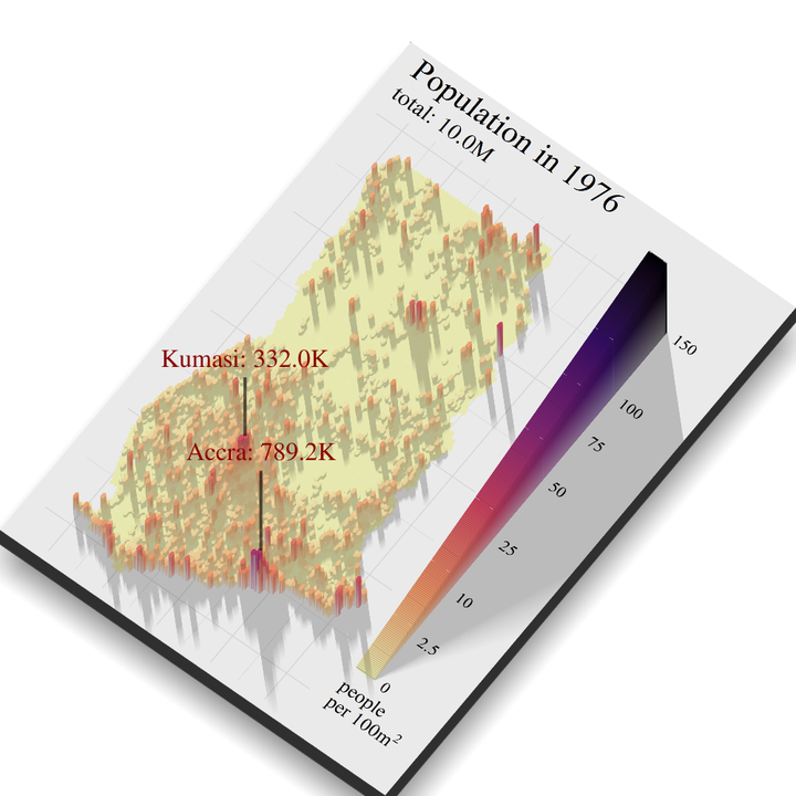
To get the population data for Kumasi and Greater Accra, I took all the points that fell in the different shapefiles of the Districts that make up these two cities. For Kumasi those districts were KMA and Asokore Mampong Municipal and For Greater Accra Accra Metropolis, La Dade Kotopon, Ga South, Ga West, Ga Central Municipal, Ga East, La Nkwantanang Madina, and Adenta. This code is quite long, and as this is a blog and not a book I am not going to fully explain every step. However, the basic idea is as follows
- Think about a scene of the animation, what happens in this scene and how long it should take.
- Define the number of frames of this scene and
for loopover all the frames in this scene and save every frame as a .png file. This gives the flexibility to stop the rendering and continuing it later. - Use the program
ffmpegto render all the frames (1575 in total) to a .mp4 file.
See here the end result (hosted on Vimeo).
## 1: download the 1990 and 2000 data tiles
grid_for_downloads <- expand.grid(year = c(1990, 2000), x = c(17, 18), y = c(7, 8))
for(i in 1:nrow(grid_for_downloads)){
data_url <- paste0("http://cidportal.jrc.ec.europa.eu/ftp/jrc-opendata/GHSL/GHS_POP_MT_GLOBE_R2019A/GHS_POP_E",
grid_for_downloads$year[i],
"_GLOBE_R2019A_54009_250/V1-0/tiles/GHS_POP_E",
grid_for_downloads$year[i],
"_GLOBE_R2019A_54009_250_V1_0_",
grid_for_downloads$x[i],
"_",
grid_for_downloads$y[i],
".zip" )
temp <- tempfile()
download.file(data_url, temp)
unzip(temp)
unlink(temp)
print(i)
}
# 1990
pop_250_m_tile_1_1990 <- raster(x = "GHS_POP_E1990_GLOBE_R2019A_54009_250_V1_0_17_7.tif")
pop_250_m_tile_2_1990 <- raster(x = "GHS_POP_E1990_GLOBE_R2019A_54009_250_V1_0_17_8.tif")
pop_250_m_tile_3_1990 <- raster(x = "GHS_POP_E1990_GLOBE_R2019A_54009_250_V1_0_18_7.tif")
pop_250_m_tile_4_1990 <- raster(x = "GHS_POP_E1990_GLOBE_R2019A_54009_250_V1_0_18_8.tif")
list_tiles_1990 <- list(pop_250_m_tile_1_1990,
pop_250_m_tile_2_1990,
pop_250_m_tile_3_1990,
pop_250_m_tile_4_1990)
West_africa_pop_1990<- do.call(merge,
list_tiles_1990)
Ghana_pop_250m_1990 <- crop(West_africa_pop_1990,
extent(as_Spatial(st_transform(Ghana_map,
crs = crs(West_africa_pop_1990)))))
Ghana_pop_250m_1990 <- mask(Ghana_pop_250m_1990,
as_Spatial(st_transform(Ghana_map,
crs = crs(West_africa_pop_1990))))
# 2000
pop_250_m_tile_1_2000 <- raster(x = "GHS_POP_E2000_GLOBE_R2019A_54009_250_V1_0_17_7.tif")
pop_250_m_tile_2_2000 <- raster(x = "GHS_POP_E2000_GLOBE_R2019A_54009_250_V1_0_17_8.tif")
pop_250_m_tile_3_2000 <- raster(x = "GHS_POP_E2000_GLOBE_R2019A_54009_250_V1_0_18_7.tif")
pop_250_m_tile_4_2000 <- raster(x = "GHS_POP_E2000_GLOBE_R2019A_54009_250_V1_0_18_8.tif")
list_tiles_2000 <- list(pop_250_m_tile_1_2000,
pop_250_m_tile_2_2000,
pop_250_m_tile_3_2000,
pop_250_m_tile_4_2000)
West_africa_pop_2000 <- do.call(merge, list_tiles_2000)
Ghana_pop_250m_2000 <- crop(West_africa_pop_2000,
extent(as_Spatial(st_transform(Ghana_map,
crs = crs(West_africa_pop_2000)))))
Ghana_pop_250m_2000 <- mask(Ghana_pop_250m_2000,
as_Spatial(st_transform(Ghana_map,
crs = crs(West_africa_pop_2000))))
## 2: load in all the data for 1975, 1990, 2000 and 2015
points_Ghana_1975 <- as_tibble(raster::rasterToPoints(Ghana_pop_250m_1975)) %>%
mutate(layer = ifelse(layer < 0, NA, layer )) %>%
rowid_to_column() %>%
mutate(year= ymd(19750101))
points_Ghana_1990 <- as_tibble(raster::rasterToPoints(Ghana_pop_250m_1990)) %>%
mutate(layer = ifelse(layer < 0, NA, layer )) %>%
rowid_to_column()%>%
mutate(year= ymd(19900101))
points_Ghana_2000 <- as_tibble(raster::rasterToPoints(Ghana_pop_250m_2000)) %>%
mutate(layer = ifelse(layer < 0, NA, layer )) %>%
rowid_to_column() %>%
mutate(year= ymd(20000101))
points_Ghana_2015 <- as_tibble(raster::rasterToPoints(Ghana_pop_250m_2015)) %>%
mutate(layer = ifelse(layer < 0, NA, layer )) %>%
rowid_to_column()%>%
mutate(year= ymd(20150101))
# -------- SCENE 1 -------- #
# the start
# from top view to adding shadows
# number of frames for scene 1
n_frames_1 <- 60
# theta values for scene 1
theta_val_1 <- seq(40, -50, length.out = n_frames_1)
# phi values for scene 1
phi_val_1 <- 50 + 15 * cos(seq(0, 360, length.out = n_frames_1) * pi /180)
# light angle values for scene 1
anglebreaks_1 <- seq(85, 30, length.out = n_frames_1)
anglebreaks_2 <- seq(95, 40, length.out = n_frames_1)
# create a 2d map
plot_out_start <- points_Ghana_1975 %>%
ggplot(aes(x = x, y = y, z = layer/(250^2/100^2))) + # the data comes in 250m*250m tiles so we recalculate that to 100m2
stat_summary_hex(bins = 70, size = 0.5) +
scale_fill_viridis_c(option = "magma",
trans = 'sqrt',
direction = -1,
limits = c(0, 150),
breaks = c(0,2.5, 10, 25, 50, 75, 100, 150),
labels = c("0", "2.5","10", "25", "50",'75', "100", "150" )) +
theme_minimal() +
coord_quickmap() +
labs(x = NULL,
y = NULL,
fill = expression(paste("people\nper 100",m^2), sep = ""),
title = "Population in 1975",
subtitle = paste0("total: ", label_number_si(accuracy=0.1)(sum(points_Ghana_1975$layer)))) +
theme(axis.text = element_blank(),
legend.position = "right",
legend.title = element_text(size = 15,
family = "serif",
margin = margin(t = .5, unit = "cm")),
legend.text = element_text(size = 13,
family = "serif"),
legend.title.align = 1,
legend.key.height = unit(5,"line"),
plot.title = element_text(family = "serif", size = 25),
plot.subtitle = element_text(family = "serif", size = 18)) +
guides(fill = guide_colourbar(title.position="bottom"))
# loop over the frames and save them 1 by 1
for(i in 1:n_frames_1){
plot_gg(plot_out_start,
multicore = TRUE,
raytrace = TRUE,
width = 5,
height = 7,
anglebreaks = seq(anglebreaks_1[i], anglebreaks_2[i], 0.1),
scale = 500,
windowsize = c(1000, 1000),
zoom = 0.8,
save_height_matrix = F,
theta = 0,
phi = 90)
Sys.sleep(.2)
# render the snap shot
render_snapshot(clear = TRUE, filename=paste0("frames/frame_",stringr::str_pad(i, 5, pad = "0"), ".png"))
# close the rgl window before renting a new frame
rgl::rgl.close()
print(i)
}
# -------- SCENE 2 -------- #
# change phi and theta
# This makes the map actually look 3 dimensional
n_frames_2 <- 60
theta_val_1 <- seq(0, 40, length.out = n_frames_2)
phi_val_1 <- seq(90, 65, length.out = n_frames_2)
# save the shadow matrix to speed up the process considerably
shadow_matrix <- plot_gg(plot_out_start,
multicore = TRUE,
raytrace = TRUE,
width = 5,
height = 7,
anglebreaks = seq(30,40, 0.1),
scale = 500,
windowsize = c(1000, 1000),
zoom = 0.8,
save_shadow_matrix = T,
theta = 0,
phi = 90)
rgl::rgl.close()
for(i in 1:n_frames_2){
plot_gg(plot_out_start,
multicore = TRUE,
raytrace = TRUE,
width = 5,
height = 7,
anglebreaks = seq(30,40, 0.1),
scale = 500,
windowsize = c(1000, 1000),
zoom = 0.8,
saved_shadow_matrix = shadow_matrix,
theta = theta_val_1[i],
phi = phi_val_1[i])
Sys.sleep(.2)
render_snapshot(clear = TRUE,
filename = paste0("frames/frame_",
stringr::str_pad(i + n_frames_1, 5, pad = "0"),
".png"))
rgl::rgl.close()
print(i)
}
# -------- SCENE 3 -------- #
# add label line for Accra and Kumasi
n_frames_3 <- 45
z_val_Kumasi <- seq(175, 600, length.out = n_frames_3)
z_val_Accra <- seq(200, 800, length.out = n_frames_3)
# this can potentially be sped up, using the saved_shadow_matrix function
height_matrix <- plot_gg(plot_out_start,
multicore = TRUE,
raytrace = TRUE,
width = 5,
height = 7,
anglebreaks = seq(30,40, 0.1),
scale = 500,
windowsize = c(1000, 1000),
zoom = 0.8,
save_height_matrix = T,
theta = 40,
phi = 65)
rgl::rgl.close()
for(i in 1:n_frames_3){
plot_gg(plot_out_start,
multicore = TRUE,
raytrace = TRUE,
saved_shadow_matrix = shadow_matrix,
width = 5,
height = 7,
anglebreaks = seq(30,40, 0.1),
scale = 500,
windowsize = c(1000, 1000),
zoom = 0.8,
theta = 40,
phi = 65)
render_label(height_matrix,
x = 460,
y = 1450,
z =z_val_Kumasi[i],
textcolor = "darkred",
linecolor = "black",
family = "serif",
text = "",
dashed = F,
linewidth = 4,
textsize = 3,
alpha = .6)
render_label(height_matrix,
x = 750,
y = 1750,
z =z_val_Accra[i],
textcolor = "darkred",
linecolor = "black",
family = "serif",
text = "",
dashed = F,
linewidth = 4,
textsize = 3,
alpha = .6)
Sys.sleep(.3)
render_snapshot(clear = TRUE,
filename = paste0("frames/frame_",
stringr::str_pad(1 + n_frames_1 + n_frames_2 + n_frames_3, 5, pad = "0"),
".png"))
rgl::rgl.close()
print(i)
}
# -------- SCENE 4 -------- #
# add Kumasi and Accra label with their population totals
# First I need to find which of the raster points fall within Accra and Kumasi
# to do this I download the district shape files for the 216 districts in Ghana
# I downloaded the shapefiles here: https://data.gov.gh/dataset/shapefiles-all-districts-ghana-2012-216-districts/resource/c89cf6a0-ef51-40fc-860d
Ghana_districts <- read_sf("district216_shapes/Map_of_Districts_216.shp", layer= "Map_of_Districts_216")
Ghana_districts <- st_transform(Ghana_districts, crs = "epsg:2136")
# Now define the cities of Accra and Kumasi
Accra_boundary <- Ghana_districts %>% filter(NAME %in% c("Accra Metropolis",
"La Dade Kotopon",
"Ga South",
"Ga West",
"Ga Central Municipal",
"Ga East",
"La Nkwantanang Madina",
"Adenta"))
Kumasi_boundary <- Ghana_districts %>% filter(NAME %in% c("Kma",
"Asokore Mampong Municipal"))
# change the points file into a sf shapefile
dat_1975_shapefile <- st_as_sf(points_Ghana_1975,
coords = c("x", "y"),
crs = crs(Ghana_pop_250m_1975)) %>%
st_transform(crs = "epsg:2136")
# check which of the 3M+ points fall in the districts that make up Accra and Kumas
intersection_Accra <- st_intersects(dat_1975_shapefile, Accra_boundary)
intersection_kumasi <- st_intersects(dat_1975_shapefile, Kumasi_boundary)
# save the number row identifiers of these points
row_ids_Accra <- points_Ghana_1975$rowid[!is.na(as.numeric(intersection_Accra))]
row_ids_Kumasi <- points_Ghana_1975$rowid[!is.na(as.numeric(intersection_kumasi))]
# create a summary of the number of people in Accra and Kumasil
summary_n_people <- points_Ghana_1975 %>%
summarise(n_people_Accra = sum(layer[rowid %in% row_ids_Accra]),
n_people_Kumasi = sum(layer[rowid %in% row_ids_Kumasi]))
# make a plot with Kumasi and Accra labels and the number of people living there in 1975
# This is just a still frame I repeat for a 15 frames
n_frames_4 <- 15
plot_gg(plot_out_start,
multicore = TRUE,
raytrace = TRUE,
saved_shadow_matrix = shadow_matrix,
width = 5,
height = 7,
anglebreaks = seq(30,40, 0.1),
scale = 500,
windowsize = c(1000, 1000),
zoom = 0.8,
theta = 40,
phi = 65)
render_label(height_matrix, x = 460, y = 1450, z =600 , textcolor = "darkred", linecolor = "black", family = "serif",
text = paste0("Kumasi: ", label_number_si(accuracy=0.1)(summary_n_people$n_people_Kumasi)) , dashed = F, linewidth = 4, textsize = 2, alpha = .6
#dashlength = 30, relativez =F,adjustvec = c(-1,-12)
)
render_label(height_matrix, x = 750, y = 1750, z =800 , textcolor = "darkred", linecolor = "black", family = "serif",
text =paste0("Accra: ", label_number_si(accuracy=0.1)(summary_n_people$n_people_Accra)), dashed = F, linewidth = 4, textsize = 2, alpha = .6
#dashlength = 30, relativez =F, adjustvec = c(-1,12)
)
Sys.sleep(.3)
render_snapshot(clear = TRUE,
filename = paste0("frames/frame_",
stringr::str_pad(1 + n_frames_1 + n_frames_2 + n_frames_3, 5, pad = "0"),
".png"))
rgl::rgl.close()
for(i in 2:n_frames_4) {
file.copy(
from = paste0(
"frames/frame_",
stringr::str_pad(1 + n_frames_1 + n_frames_2 + n_frames_3, 5, pad = "0"),
".png"
),
to = paste0(
"frames/frame_",
stringr::str_pad(i + n_frames_1 + n_frames_2 + n_frames_3, 5, pad = "0"),
".png"
)
)
}
# -------- SCENE 5 -------- #
# animate data from 1975 to 1990
# first interpolate the data from 1975 to 1990
# and fill in the data for 1976 to 1989 for which no data is available
data_1975_1990_by_year_inter <-
tibble(
rowid = rep(points_Ghana_1975$rowid, 16),
x = rep(points_Ghana_1975$x, 16),
y = rep(points_Ghana_1975$y, 16),
layer = c(
points_Ghana_1975$layer,
rep(NA, 14 * nrow(points_Ghana_1975)),
points_Ghana_1990$layer
),
year = rep(seq(ymd(19750101),
ymd(19900101),
"year"),
each = nrow(points_Ghana_1975))
) %>%
group_by(rowid) %>%
mutate(layer = zoo::na.approx(layer))
# summarise this data into national (interpolated ) totals
# and totals for Accra and Kumasi fro 1975 to 1990
titles_1975_1990 <- data_1975_1990_by_year_inter %>%
group_by(year ) %>%
summarise(tot = sum(layer),
n_people_Accra = sum(layer[rowid %in% row_ids_Accra]),
n_people_Kumasi = sum(layer[rowid %in% row_ids_Kumasi]))
# I do 30 frames per year
frames_per_year <- 30
n_frames_total <- 40 * frames_per_year
theta_val_2 <- seq(40,-50, length.out = n_frames_total)
phi_val_2 <-
50 + 15 * cos(seq(0, 360, length.out = n_frames_total) * pi / 180)
#
years_1975_1990 <- seq(ymd(19750101),
ymd(19900101),
"year")
gc() # Clean the ram
for (i in 1:(length(years_1975_1990) - 1)) {
# In addition to the interpolation between years
# I also tween data within years, This way the animation is butter smooth
# basically, the change from year to year is split up in 40 frames of animation
# year t
dat_begin <- data_1975_1990_by_year_inter %>%
ungroup() %>%
filter(year == years_1975_1990[i])
# year t+1
dat_end <- data_1975_1990_by_year_inter %>%
ungroup() %>%
filter(year == years_1975_1990[i + 1])
# tween data linearly
dat <- tween_states(
data = list(dat_begin, dat_end),
tweenlength = 1,
statelength = 0,
ease = 'linear',
nframes = frames_per_year
)
# clean some memory space
# you might want to clean some other objects from your R Enviromemt
rm(dat_begin)
rm(dat_end)
for (j in 1:frames_per_year) {
plot_out <- dat %>%
filter(.frame == j) %>%
ggplot(aes(
x = x,
y = y,
z = layer / (250 ^ 2 / 100 ^ 2)
)) + # the data comes in 250m*250m tiles so we recalculate that to 100m2
stat_summary_hex(bins = 70, size = 0.5) +
scale_fill_viridis_c(
option = "magma",
trans = 'sqrt',
direction = -1,
limits = c(0, 150),
breaks = c(0, 2.5, 10, 25, 50, 75, 100, 150),
labels = c("0", "2.5", "10", "25", "50", '75', "100", "150")
) +
theme_minimal() +
coord_quickmap() +
labs(
x = NULL,
y = NULL,
fill = expression(paste("people\nper 100", m ^ 2), sep = ""),
title = paste0("Population in ", year(years_1975_1990[i])),
subtitle = paste0(
"total: ",
label_number_si(accuracy = 0.1)(titles_1975_1990$tot[i])
)
) +
theme(
axis.text = element_blank(),
legend.position = "right",
legend.title = element_text(
size = 15,
family = "serif",
margin = margin(t = .5, unit = "cm")
),
legend.text = element_text(size = 13,
family = "serif"),
legend.title.align = 1,
legend.key.height = unit(5, "line"),
plot.title = element_text(family = "serif", size = 25),
plot.subtitle = element_text(family = "serif", size = 18)
) +
guides(fill = guide_colourbar(title.position = "bottom"))
height_matrix <- plot_gg(
plot_out,
multicore = TRUE,
raytrace = T,
width = 5,
height = 7,
scale = 500,
windowsize = c(1000, 1000),
zoom = 0.8,
save_height_matrix = TRUE,
theta = theta_val_2[j + ((i - 1) * frames_per_year)],
phi = phi_val_2[j + ((i - 1) * frames_per_year)]
)
render_label(
height_matrix,
x = 460,
y = 1450,
z = 600 ,
textcolor = "darkred",
linecolor = "black",
family = "serif",
text = paste0(
"Kumasi: ",
ifelse(
titles_1975_1990$n_people_Kumasi[i] < 1e6 ,
label_number_si(accuracy =
0.1)(titles_1975_1990$n_people_Kumasi[i]),
label_number_si(accuracy =
0.01)(titles_1975_1990$n_people_Kumasi[i])
)
),
dashed = F,
linewidth = 4,
textsize = 2,
alpha = .6
)
render_label(
height_matrix,
x = 750,
y = 1750,
z = 800 ,
textcolor = "darkred",
linecolor = "black",
family = "serif",
text = paste0(
"Accra: ",
ifelse(
titles_1975_1990$n_people_Accra[i] < 1e6 ,
label_number_si(accuracy =
0.1)(titles_1975_1990$n_people_Accra[i]),
label_number_si(accuracy =
0.01)(titles_1975_1990$n_people_Accra[i])
)
),
dashed = F,
linewidth = 4,
textsize = 2,
alpha = .6
)
Sys.sleep(.2)
render_snapshot(
clear = TRUE,
filename = paste0(
"frames/frame_",
stringr::str_pad(
j +
n_frames_1 +
n_frames_2 +
n_frames_3 +
n_frames_4 +
((i -
1) * frames_per_year),
5,
pad = "0"
),
".png"
)
)
rgl::rgl.close()
rm(plot_out)
rm(height_matrix)
gc() # clean the RAM
print(paste0("frame: ", j, " out of ", frames_per_year))
}
rm(dat)
print(paste0("year: ", i, " out of ", (length(years_1975_1990) - 1)))
}
# -------- SCENE 6 -------- #
# animate data from 1990 to 2000
# This code follows the exact same steps as scene 5, but now for the period 1990 to 2000
data_1990_2000_by_year_inter <-
tibble(
rowid = rep(points_Ghana_1990$rowid, 11),
x = rep(points_Ghana_1990$x, 11),
y = rep(points_Ghana_1990$y, 11),
layer = c(
points_Ghana_1990$layer,
rep(NA, 9 * nrow(points_Ghana_1990)),
points_Ghana_2000$layer
),
year = rep(seq(ymd(19900101),
ymd(20000101),
"year"),
each = nrow(points_Ghana_1990))
) %>%
group_by(rowid) %>%
mutate(layer = zoo::na.approx(layer))
data_1990_2000_by_year_inter %>%
group_by(year) %>%
summarise(n = n())
titles_1990_2000 <- data_1990_2000_by_year_inter %>%
group_by(year) %>%
summarise(
tot = sum(layer),
n_people_Accra = sum(layer[rowid %in% row_ids_Accra]),
n_people_Kumasi = sum(layer[rowid %in% row_ids_Kumasi])
)
years_1990_2000 <- seq(ymd(19900101),
ymd(20000101),
"year")
gdata::keep(
n_frames_1,
n_frames_2,
n_frames_3,
n_frames_4,
frames_per_year,
n_frames_total,
theta_val_2,
phi_val_2,
years_1990_2000,
data_1990_2000_by_year_inter,
titles_1990_2000,
row_ids_Accra,
row_ids_Kumasi,
sure = T
)
z_val_Accra_2 <- c(seq(800, 700, length.out = 2 * frames_per_year),
rep(rep(700, frames_per_year), each = 8))
for (i in 1:(length(years_1990_2000) - 1)) {
dat_begin <- data_1990_2000_by_year_inter %>%
ungroup() %>%
filter(year == years_1990_2000[i])
dat_end <- data_1990_2000_by_year_inter %>%
ungroup() %>%
filter(year == years_1990_2000[i + 1])
dat <- tween_states(
data = list(dat_begin, dat_end),
tweenlength = 1,
statelength = 0,
ease = 'linear',
nframes = frames_per_year
)
rm(dat_begin)
rm(dat_end)
for (j in 1:frames_per_year) {
plot_out <- dat %>%
filter(.frame == j) %>%
ggplot(aes(
x = x,
y = y,
z = layer / (250 ^ 2 / 100 ^ 2)
)) + # the data comes in 250m*250m tiles so we recalculate that to 100m2
stat_summary_hex(bins = 70, size = 0.5) +
scale_fill_viridis_c(
option = "magma",
trans = 'sqrt',
direction = -1,
limits = c(0, 150),
breaks = c(0, 2.5, 10, 25, 50, 75, 100, 150),
labels = c("0", "2.5", "10", "25", "50", '75', "100", "150")
) +
theme_minimal() +
coord_quickmap() +
labs(
x = NULL,
y = NULL,
fill = expression(paste("people\nper 100", m ^ 2), sep = ""),
title = paste0("Population in ", year(years_1990_2000[i])),
subtitle = paste0(
"total: ",
label_number_si(accuracy = 0.1)(titles_1990_2000$tot[i])
)
) +
theme(
axis.text = element_blank(),
legend.position = "right",
legend.title = element_text(
size = 15,
family = "serif",
margin = margin(t = .5, unit = "cm")
),
legend.text = element_text(size = 13,
family = "serif"),
legend.title.align = 1,
legend.key.height = unit(5, "line"),
plot.title = element_text(family = "serif", size = 25),
plot.subtitle = element_text(family = "serif", size = 18)
) +
guides(fill = guide_colourbar(title.position = "bottom"))
height_matrix <- plot_gg(
plot_out,
multicore = TRUE,
raytrace = T,
width = 5,
height = 7,
scale = 500,
windowsize = c(1000, 1000),
zoom = 0.8,
save_height_matrix = TRUE,
theta = theta_val_2[j + ((i - 1) * frames_per_year) + ((1990 - 1975) * frames_per_year)],
phi = phi_val_2[j + ((i - 1) * frames_per_year) + ((1990 - 1975) * frames_per_year)]
)
render_label(
height_matrix,
x = 460,
y = 1450,
z = 600 ,
textcolor = "darkred",
linecolor = "black",
family = "serif",
text = paste0(
"Kumasi: ",
ifelse(
titles_1990_2000$n_people_Kumasi[i] < 1e6 ,
label_number_si(accuracy =
0.1)(titles_1990_2000$n_people_Kumasi[i]),
label_number_si(accuracy =
0.01)(titles_1990_2000$n_people_Kumasi[i])
)
),
dashed = F,
linewidth = 4,
textsize = 2,
alpha = .6
)
render_label(
height_matrix,
x = 750,
y = 1750,
z = z_val_Accra_2[((i - 1) * frames_per_year + j)],
textcolor = "darkred",
linecolor = "black",
family = "serif",
text = paste0(
"Accra: ",
ifelse(
titles_1990_2000$n_people_Accra[i] < 1e6 ,
label_number_si(accuracy =
0.1)(titles_1990_2000$n_people_Accra[i]),
label_number_si(accuracy =
0.01)(titles_1990_2000$n_people_Accra[i])
)
),
dashed = F,
linewidth = 4,
textsize = 2,
alpha = .6
)
Sys.sleep(.4)
render_snapshot(
clear = TRUE,
filename = paste0(
"frames/frame_",
stringr::str_pad(
j +
n_frames_1 +
n_frames_2 +
n_frames_3 +
n_frames_4 +
((1990 - 1975) * frames_per_year) +
((i -
1) * frames_per_year),
5,
pad = "0"
),
".png"
)
)
rgl::rgl.close()
rm(plot_out)
rm(height_matrix)
gc()
print(paste0("frame: ", j, " out of ", frames_per_year))
}
rm(dat)
print(paste0("year: ", i, " out of ", (length(years_1990_2000) - 1)))
}
# -------- SCENE 7 -------- #
# animate data from 2000 to 2015
data_2000_2015_by_year_inter <-
tibble(
rowid = rep(points_Ghana_2000$rowid, 16),
x = rep(points_Ghana_2000$x, 16),
y = rep(points_Ghana_2000$y, 16),
layer = c(
points_Ghana_2000$layer,
rep(NA, 14 * nrow(points_Ghana_2000)),
points_Ghana_2015$layer
),
year = rep(seq(ymd(20000101),
ymd(20150101),
"year"),
each = nrow(points_Ghana_2000))
) %>%
group_by(rowid) %>%
mutate(layer = zoo::na.approx(layer))
data_2000_2015_by_year_inter %>%
group_by(year) %>%
summarise(n = n())
titles_2000_2015 <- data_2000_2015_by_year_inter %>%
group_by(year) %>%
summarise(
tot = sum(layer),
n_people_Accra = sum(layer[rowid %in% row_ids_Accra]),
n_people_Kumasi = sum(layer[rowid %in% row_ids_Kumasi])
)
years_2000_2015 <- seq(ymd(20000101),
ymd(20150101),
"year")
z_val_Accra_3 <- c(rep(rep(700, frames_per_year), each = 3),
seq(700, 650, length.out = 2 * frames_per_year),
rep(rep(650, frames_per_year), each = 10))
# The height label of Kumasi needs to bounce a bit,
# to make sure it does not overlap with the Accra label
z_val_Kumasi_2 <- c(
rep(rep(600, frames_per_year), each = 5),
seq(600, 674.7492, length.out = 5 * frames_per_year),
seq(674.7492, 850, length.out = 5 * frames_per_year)
)
for (i in 1:(length(years_2000_2015) - 1)) {
dat_begin <- data_2000_2015_by_year_inter %>%
ungroup() %>%
filter(year == years_2000_2015[i])
dat_end <- data_2000_2015_by_year_inter %>%
ungroup() %>%
filter(year == years_2000_2015[i + 1])
dat <- tween_states(
data = list(dat_begin, dat_end),
tweenlength = 1,
statelength = 0,
ease = 'linear',
nframes = frames_per_year
)
rm(dat_begin)
rm(dat_end)
for (j in 1:frames_per_year) {
plot_out <- dat %>%
filter(.frame == j) %>%
ggplot(aes(
x = x,
y = y,
z = layer / (250 ^ 2 / 100 ^ 2)
)) + # the data comes in 250m*250m tiles so we recalculate that to 100m2
stat_summary_hex(bins = 70, size = 0.5) +
scale_fill_viridis_c(
option = "magma",
trans = 'sqrt',
direction = -1,
limits = c(0, 150),
breaks = c(0, 2.5, 10, 25, 50, 75, 100, 150),
labels = c("0", "2.5", "10", "25", "50", '75', "100", "150")
) +
theme_minimal() +
coord_quickmap() +
labs(
x = NULL,
y = NULL,
fill = expression(paste("people\nper 100", m ^ 2), sep = ""),
title = paste0("Population in ", year(years_2000_2015[i])),
subtitle = paste0(
"total: ",
label_number_si(accuracy = 0.1)(titles_2000_2015$tot[i])
)
) +
theme(
axis.text = element_blank(),
legend.position = "right",
legend.title = element_text(
size = 15,
family = "serif",
margin = margin(t = .5, unit = "cm")
),
legend.text = element_text(size = 13,
family = "serif"),
legend.title.align = 1,
legend.key.height = unit(5, "line"),
plot.title = element_text(family = "serif", size = 25),
plot.subtitle = element_text(family = "serif", size = 18)
) +
guides(fill = guide_colourbar(title.position = "bottom"))
height_matrix <- plot_gg(
plot_out,
multicore = TRUE,
raytrace = T,
width = 5,
height = 7,
scale = 500,
windowsize = c(1000, 1000),
zoom = 0.8,
save_height_matrix = TRUE,
theta = theta_val_2[j + ((i - 1) * frames_per_year) + ((2000 - 1975) * frames_per_year)],
phi = phi_val_2[j + ((i - 1) * frames_per_year) + ((2000 - 1975) * frames_per_year)]
)
render_label(
height_matrix,
x = 460,
y = 1450,
z = z_val_Kumasi_2[((i - 1) * frames_per_year + j)],
textcolor = "darkred",
linecolor = "black",
family = "serif",
relativez = F,
text = paste0(
"Kumasi: ",
ifelse(
titles_2000_2015$n_people_Kumasi[i] < 1e6 ,
label_number_si(accuracy =
0.1)(titles_2000_2015$n_people_Kumasi[i]),
label_number_si(accuracy =
0.01)(titles_2000_2015$n_people_Kumasi[i])
)
),
dashed = F,
linewidth = 4,
textsize = 2,
alpha = .6
)
render_label(
height_matrix,
x = 750,
y = 1750,
z = z_val_Accra_3[((i - 1) * frames_per_year + j)],
textcolor = "darkred",
linecolor = "black",
family = "serif",
relativez = F,
text = paste0(
"Accra: ",
ifelse(
titles_2000_2015$n_people_Accra[i] < 1e6 ,
label_number_si(accuracy =
0.1)(titles_2000_2015$n_people_Accra[i]),
label_number_si(accuracy =
0.01)(titles_2000_2015$n_people_Accra[i])
)
),
dashed = F,
linewidth = 4,
textsize = 2,
alpha = .6
)
Sys.sleep(.2)
render_snapshot(
clear = TRUE,
filename = paste0(
"frames/frame_",
stringr::str_pad(
j +
n_frames_1 +
n_frames_2 +
n_frames_3 +
n_frames_4 +
((2000 - 1975) * frames_per_year) +
((i -
1) * frames_per_year),
5,
pad = "0"
),
".png"
)
)
rgl::rgl.close()
rm(plot_out)
rm(height_matrix)
gc()
print(paste0("frame: ", j, " out of ", frames_per_year))
}
rm(dat)
print(paste0("year: ", i, " out of ", (length(years_2000_2015) - 1)))
}
# -------- SCENE 8 -------- #
# Freeze the final frame for the year 2015 for 15 frames
n_frames_6 <- 15
summary_n_people <- points_Ghana_2015 %>%
summarise(n_people_Accra = sum(layer[rowid %in% row_ids_Accra]),
n_people_Kumasi = sum(layer[rowid %in% row_ids_Kumasi]))
plot_out_end <- points_Ghana_2015 %>%
ggplot(aes(
x = x,
y = y,
z = layer / (250 ^ 2 / 100 ^ 2)
)) +
stat_summary_hex(bins = 70, size = 0.5) +
scale_fill_viridis_c(
option = "magma",
trans = 'sqrt',
direction = -1,
limits = c(0, 150),
breaks = c(0, 2.5, 10, 25, 50, 75, 100, 150),
labels = c("0", "2.5", "10", "25", "50", '75', "100", "150")
) +
theme_minimal() +
coord_quickmap() +
labs(
x = NULL,
y = NULL,
fill = expression(paste("people\nper 100", m ^ 2), sep = ""),
title = "Population in 2015",
subtitle = paste0("total: ", label_number_si(accuracy = 0.1)(sum(
points_Ghana_2015$layer
)))
) +
theme(
axis.text = element_blank(),
legend.position = "right",
legend.title = element_text(
size = 15,
family = "serif",
margin = margin(t = .5, unit = "cm")
),
legend.text = element_text(size = 13,
family = "serif"),
legend.title.align = 1,
legend.key.height = unit(5, "line"),
plot.title = element_text(family = "serif", size = 25),
plot.subtitle = element_text(family = "serif", size = 18)
) +
guides(fill = guide_colourbar(title.position = "bottom"))
shadow_matrix_end <- plot_gg(
plot_out_end,
multicore = TRUE,
raytrace = TRUE,
width = 5,
height = 7,
anglebreaks = seq(30, 40, 0.1),
scale = 500,
windowsize = c(1000, 1000),
zoom = 0.8,
save_shadow_matrix = T,
theta = -50,
phi = 65
)
height_matrix_end <- plot_gg(
plot_out_end,
multicore = TRUE,
raytrace = TRUE,
saved_shadow_matrix = shadow_matrix_end,
width = 5,
height = 7,
anglebreaks = seq(30, 40, 0.1),
scale = 500,
windowsize = c(1000, 1000),
save_height_matrix = TRUE,
zoom = 0.8,
theta = -50,
phi = 65
)
render_label(
height_matrix_end,
x = 460,
y = 1450,
z = 850 ,
textcolor = "darkred",
linecolor = "black",
family = "serif",
text = paste0(
"Kumasi: ",
label_number_si(accuracy = 0.01)(summary_n_people$n_people_Kumasi)
) ,
dashed = F,
linewidth = 4,
textsize = 2,
alpha = .6
)
render_label(
height_matrix_end,
x = 750,
y = 1750,
z = 650 ,
textcolor = "darkred",
linecolor = "black",
family = "serif",
text = paste0(
"Accra: ",
label_number_si(accuracy = 0.01)(summary_n_people$n_people_Accra)
),
dashed = F,
linewidth = 4,
textsize = 2,
alpha = .6
)
Sys.sleep(.3)
render_snapshot(clear = TRUE,
filename = paste0(
"frames/frame_",
stringr::str_pad(
1 +
n_frames_1 +
n_frames_2 +
n_frames_3 +
n_frames_4 +
((2015 - 1975) * frames_per_year),
5,
pad = "0"
),
".png"
))
rgl::rgl.close()
for (i in 2:n_frames_6) {
file.copy(
from = paste0(
"frames/frame_",
stringr::str_pad(
1 +
n_frames_1 +
n_frames_2 +
n_frames_3 +
n_frames_4 +
((2015 - 1975) * frames_per_year),
5,
pad = "0"
),
".png"
),
to = paste0(
"frames/frame_",
stringr::str_pad(
i +
n_frames_1 +
n_frames_2 +
n_frames_3 +
n_frames_4 +
((2015 - 1975) * frames_per_year),
5,
pad = "0"
),
".png"
)
)
}
# -------- SCENE 9 -------- #
# Make the labels for Kumasi and Accra disappear
n_frames_7 <- 60
z_val_Kumasi_4 <- seq(850, 100, length.out = n_frames_7)
z_val_Accra_4 <- seq(650, 100, length.out = n_frames_7)
size_val <- seq(2, 0, length.out = n_frames_7)
for (i in 1:n_frames_7) {
plot_gg(
plot_out_end,
multicore = TRUE,
raytrace = TRUE,
saved_shadow_matrix = shadow_matrix_end,
width = 5,
height = 7,
anglebreaks = seq(30, 40, 0.1),
scale = 500,
windowsize = c(1000, 1000),
zoom = 0.8,
theta = -50,
phi = 65
)
render_label(
height_matrix_end,
x = 460,
y = 1450,
z = z_val_Kumasi_4[i] ,
textcolor = "darkred",
linecolor = "black",
family = "serif",
text = paste0(
"Kumasi: ",
label_number_si(accuracy = 0.01)(summary_n_people$n_people_Kumasi)
),
dashed = F,
linewidth = 4,
textsize = size_val[i],
alpha = .6
)
render_label(
height_matrix_end,
x = 750,
y = 1750,
z = z_val_Accra_4[i] ,
textcolor = "darkred",
linecolor = "black",
family = "serif",
text = paste0(
"Accra: ",
label_number_si(accuracy = 0.01)(summary_n_people$n_people_Accra)
),
dashed = F,
linewidth = 4,
textsize = size_val[i],
alpha = .6
)
Sys.sleep(.3)
render_snapshot(
clear = TRUE,
filename = paste0(
"frames/frame_",
stringr::str_pad(
i +
n_frames_1 +
n_frames_2 +
n_frames_3 +
n_frames_4 +
((2015 - 1975) * frames_per_year) +
n_frames_6,
5,
pad = "0"
),
".png"
)
)
rgl::rgl.close()
print(i)
}
# -------- SCENE 10 -------- #
# in 120 frames rotate to a topdown view again.
# also make sure the lighting comes from above to remove shadows.
n_frames_8 <- 120
theta_val_3 <- seq(-50, 0, length.out = n_frames_8)
phi_val_3 <- seq(65, 90, length.out = n_frames_8)
anglebreaks_1_end <- seq(30, 85, length.out = n_frames_8)
anglebreaks_2_end <- seq(40, 95, length.out = n_frames_8)
for (i in 1:n_frames_8) {
plot_gg(
plot_out_end,
multicore = TRUE,
raytrace = TRUE,
width = 5,
height = 7,
anglebreaks = seq(anglebreaks_1_end[i],
anglebreaks_2_end[i], 0.1),
scale = 500,
windowsize = c(1000, 1000),
zoom = 0.8,
save_height_matrix = F,
theta = theta_val_3[i],
phi = phi_val_3[i]
)
Sys.sleep(.2)
render_snapshot(
clear = TRUE,
filename = paste0(
"frames/frame_",
stringr::str_pad(
i +
n_frames_1 +
n_frames_2 +
n_frames_3 +
n_frames_4 +
((2015 - 1975) * frames_per_year) +
n_frames_6 +
n_frames_7,
5,
pad = "0"
),
".png"
)
)
rgl::rgl.close()
print(i)
}
####################
### -- RENDER -- ###
####################
# now I can render all the frames into in video file
system(command = "ffmpeg -framerate 45 -i frames/frame_%05d.png -c:v libx264 -vf fps=45 -pix_fmt yuv420p -crf 15 Video_Ghana_PopDens.mp4")
Correction
I realized I made a stupid calculation error. The legend title of the animation should state n people per 100x100m or n people per 10.000m$^2$, not 100m$^2$. This is dumb, but I cannot be bothered, for now, to re-render the whole animation and having a boiling hot laptop to work with for another whole day.
valuable information
These are some further valuable (re)sources, on working with raster data, making animations and the rayshader package
- https://rstudio-pubs-static.s3.amazonaws.com/297476_0d048d71ed0245b4948906958dbc53ed.html
- http://marxanconnect.ca/CF_landscape.html
- https://www.tylermw.com/getting-started-with-rayrender/
- https://twitter.com/tylermorganwall/status/1188505201193488386
- https://wcmbishop.github.io/rayshader-demo/
- https://datapleth.io/blog/2019/10/17/2019-10-17_usa_measles_map_video/
- https://publish.twitter.com/?url=https://twitter.com/tylermorganwall/status/1188099732704509953
- https://twitter.com/tylermorganwall/status/1188099732704509953
- https://medium.com/analytics-vidhya/building-a-3d-map-in-r-covid-density-in-the-us-by-income-fab409544fcb
All of these sources helped me tremendously to write this post.
Ghana Data Stuff
This website is my hobby project to showcase some of the project I am working one, when I am not working on the official statistics at the Ghana Statistical Service.