Plotting the Average Driving Time to the Nearest Hospital in Ghana

Introduction
This post in an extension of my post
on calculating the average walking time from any given location in Accra, Ghana to the nearest bar. Instead of walking times to bars this post uses the same methodology to calculate the driving time to the nearest hospital from any given point in Ghana. This involves getting data from OSM, planning walking routes and times in OSRM, plotting in cartography and ggplot2, using the sp, sf, raster, jstat, osmdata, and osrm packages.
This code took heavy inspiration and some direct code from these sources, all credit to these authors. Please have a look at what they did and some of the great tutorials they wrote:
- https://rcarto.github.io/caRtosm/index.html
- https://rpubs.com/mgei/drivingtimes
- https://www.user2019.fr/static/pres/lt257361.pdf
Packages
These are the packages used for this project:
library(tidyverse)
library(osmdata)
library(sf)
library(maptools)
library(raster)
library(RColorBrewer)
library(sp)
library(gstat)
library(osrm)
library(ggmap)
library(ggtext)
library(cartography)
library(showtext)
library(readxl)
library(fuzzyjoin)
library(chron)
library(kableExtra)

#raster overrides the dplyr select function, so assign I assigned it back
select <- dplyr::select
Data
First I needed to the find the locations of all hospitals in Ghana, a non-trivial task. The two main sources of this information are:
- A list published on https://data.gov.gh/dataset/health-facilities-ghana. This list form 2012 contains the names and locations of 3,756 different health facilities in Ghana, including health directorate offices, senior homes, CHPS clinics, and Maternity Homes. The list is almost complete, but misses some location data (longitude and latitude).
- A 2019 public database by Joseph Maina, Paul O. Ouma, Peter M. Macharia, Victor A. Alegana, Benard Mitto, Ibrahima Socé Fall, Abdisalan M. Noor, Robert W. Snow and Emelda A. Okiro, which is an Africa-wide database of Government/public hospitals. This database does not have any private hospitals (at least not in Ghana), but it has some GPS coordinates for hospitals that are missing in the first source.
Using the download.file() command I can download these files straight into my working directory
# Download first dataset
download.file("https://data.gov.gh/sites/default/files/Health%20Facility%20in%20Ghana%202012_0.csv", "dataset_GOV.csv")
# Download second dataset
download.file("https://springernature.figshare.com/ndownloader/files/14379593", "dataset_Maina.xlsx")
This is how the first dataset looks like (I am using kable tables to make the HTML tables a bit more pleasant to look at):
# load data
dat_1 <- read_csv("dataset_GOV.csv")

head(dat_1)  %>%
  kable() %>%
  kable_styling(c("striped", "hover", "condensed"))
| Region | District | Facility Name | Type | Town | Ownership | Latitude | Longitude |
|---|---|---|---|---|---|---|---|
| Ashanti | Offinso North | A.M.E Zion Clinic | Clinic | Afrancho | CHAG | 7.40801 | -1.96317 |
| Ashanti | Bekwai Municipal | Abenkyiman Clinic | Clinic | Anwiankwanta | Private | 6.46312 | -1.58592 |
| Ashanti | Adansi North | Aboabo Health Centre | Health Centre | Aboabo No 2 | Government | 6.22393 | -1.34982 |
| Ashanti | Afigya-Kwabre | Aboabogya Health Centre | Health Centre | Aboabogya | Government | 6.84177 | -1.61098 |
| Ashanti | Kwabre | Aboaso Health Centre | Health Centre | Aboaso | Government | 6.84177 | -1.61098 |
| Ashanti | Offinso North | Aboffour Health Centre | Health Centre | Aboffour | Government | 7.12986 | -1.73294 |
# table hospital types
dat_1 %>%
  group_by(Type) %>%
  count() %>%
  kable() %>%
  kable_styling(c("striped", "hover", "condensed"))
| Type | n |
|---|---|
| Centre | 2 |
| CHPS | 652 |
| clinic | 2 |
| Clinic | 1171 |
| CPHS | 1 |
| DHD | 1 |
| District Health Directorate | 99 |
| District Hospital | 82 |
| Health Centre | 786 |
| Hospital | 277 |
| Maternity Home | 369 |
| Metropolitan Health Directorate | 2 |
| Metropolitan Hospital | 1 |
| Municipal Health Directorate | 1 |
| Municipal Health Directorate | 7 |
| Municipal Hospital | 4 |
| Others | 31 |
| Polyclinic | 16 |
| Psychiatric Hospital | 3 |
| RCH | 152 |
| Regional Health Directorate | 9 |
| Regional Hospital | 9 |
| Research Institution | 2 |
| Teaching Hospital | 3 |
| Training Institution | 74 |
For this specific post I am not interested in any health facility that is not classified as a hospital, so using some regex, I can filter only for types that include the string “Hospital”, which includes the Regional Hospitals, District Hospitals.
# filter only for Hospital
dat_1 <- dat_1 %>%
  filter(grepl("Hospital", Type))

dat_1%>%
  group_by(District,  Town, `Facility Name`) %>%
  mutate(n = n()) %>%
  filter(n != 1) %>%
  arrange(`Facility Name`) %>%
  kable() %>%
  kable_styling(c("striped", "hover", "condensed"))
| Region | District | Facility Name | Type | Town | Ownership | Latitude | Longitude | n |
|---|---|---|---|---|---|---|---|---|
| Brong Ahafo | Sene | Kwame Danso Hospital | Hospital | Kwame Danso | Government | NA | NA | 2 |
| Brong Ahafo | Sene | Kwame Danso Hospital | Hospital | Kwame Danso | Government | NA | NA | 2 |
| Ashanti | Mampong Municipal | Mampong Quality Hospital | Hospital | Mampong | Private | 7.04621 | -1.40195 | 2 |
| Ashanti | Mampong Municipal | Mampong Quality Hospital | Hospital | Mampong | Private | NA | NA | 2 |
| Western | Ahanta West | Nana Hima-Dekyi Hospital | District Hospital | NA | Government | NA | NA | 2 |
| Western | Ahanta West | Nana Hima-Dekyi Hospital | District Hospital | NA | Government | NA | NA | 2 |
| Northern | Savelugu-Nanton | Savelugu Hospital | Hospital | Savelugu | Government | 9.61862 | -0.82929 | 2 |
| Northern | Savelugu-Nanton | Savelugu Hospital | District Hospital | Savelugu | Government | 9.61862 | -0.82929 | 2 |
| Brong Ahafo | Sunyani Municipal | SDA Hospital | Hospital | Sunyani | Private | NA | NA | 2 |
| Brong Ahafo | Sunyani Municipal | SDA Hospital | Hospital | Sunyani | CHAG | NA | NA | 2 |
There are some duplicates in this data I need to deal with.
# using distinct to omit duplicates
dat_1 <- dat_1 %>%
  arrange(`Facility Name`) %>%
  distinct(District, Town, `Facility Name`, .keep_all = TRUE)

nrow(dat_1)
## [1] 374
Thera are 374 hospitals left. Now I can load in the second dataset and filter for only hospitals in Ghana.
dat_2 <- read_excel("dataset_Maina.xlsx", sheet = 1) %>%
  # filter for Ghana
  filter(Country == "Ghana") %>%
  # filter for hospitals
  filter(grepl("Hospital", `Facility type`))
There is one duplicate in this dataset:
dat_2 %>%
  group_by(Admin1, `Facility name`) %>%
  mutate(n = n()) %>%
  filter(n != 1) %>%
  kable() %>%
  kable_styling(c("striped", "hover", "condensed"))
| Country | Admin1 | Facility name | Facility type | Ownership | Lat | Long | LL source | n |
|---|---|---|---|---|---|---|---|---|
| Ghana | Greater Accra | Achimota Hospital | Hospital | MoH | 5.609531 | -0.228106 | Other | 2 |
| Ghana | Greater Accra | Achimota Hospital | Hospital | MoH | 5.629220 | -0.214760 | GPS | 2 |
After some Googling, it is clear it should be the second Achimota Hospital.There are now 177 Hospitals in this dataset.
dat_2 <- dat_2 %>%
  filter(!(`Facility name` == "Achimota Hospital" & Lat == 5.609531))

glimpse(dat_2)
## Rows: 177
## Columns: 8
## $ Country         <chr> "Ghana", "Ghana", "Ghana", "Ghana", "Ghana", "Ghana...
## $ Admin1          <chr> "Ashanti", "Ashanti", "Ashanti", "Ashanti", "Ashant...
## $ `Facility name` <chr> "Agogo Presby Hospital", "Akomaa Memorial Hospital"...
## $ `Facility type` <chr> "Hospital", "Hospital", "Hospital", "Hospital", "Di...
## $ Ownership       <chr> "FBO", "FBO", "FBO", "FBO", "MoH", "MoH", "FBO", "M...
## $ Lat             <dbl> 6.796180, 6.439660, 7.053220, 6.843610, 6.801620, 6...
## $ Long            <dbl> -1.085290, -1.538370, -1.509640, -1.381201, -1.5137...
## $ `LL source`     <chr> "GPS", "GPS", "GPS", "Other", "GPS", "GPS", "GPS", ...
sum(is.na(dat_1$Latitude))
## [1] 42
A total of 42 locations are missing from the first dataset. I can join the second dataset to it to link some location data from it that is available in the second dataset, but not the first. I need to use a fuzzy-join, using the Levenstein-distance from the fuzzyjoin package, to allow for some misspellings (for example, I do want “Nkwanta Dsitrict Hospital” to match to “Nkwanta District Hospital” (typo in district in first dataset).
# match datasets
dat_complete <- dat_1 %>%
  stringdist_left_join(select(dat_2, Admin1, `Facility name`, Lat, Long),
            by = c("Facility Name" = "Facility name",
                   "Region" = "Admin1"),
            max_dist = 2,
            distance_col = "col",
            method = "lv") %>%
  mutate(Latitude  = ifelse(is.na(Latitude), Lat, Latitude),
         Longitude = ifelse(is.na(Longitude), Long, Longitude)) %>%
  select(- Lat, -Long, -`Facility Name.col`, -Region.col, -col)

# show entries that are still incomplete
dat_complete %>%
  filter(is.na(Latitude)) %>%
  kable() %>%
  kable_styling(c("striped", "hover", "condensed")) %>%
  scroll_box(width = "100%", height = "200px")
| Region | District | Facility Name | Type | Town | Ownership | Latitude | Longitude | Admin1 | Facility name |
|---|---|---|---|---|---|---|---|---|---|
| Ashanti | Kumasi Metropolitan | Abrepo County Hospital | Hospital | Abrepo | Private | NA | NA | NA | NA |
| Ashanti | Kumasi Metropolitan | Adiebeba Hospital | Hospital | Adiebeba | Private | NA | NA | NA | NA |
| Ashanti | Kumasi Metropolitan | Agyei Eli Hospital | Hospital | Sokoban | Private | NA | NA | NA | NA |
| Ashanti | Kumasi Metropolitan | Ahodwo Washie Hospital | Hospital | Ahodwo | Private | NA | NA | NA | NA |
| Ashanti | Kumasi Metropolitan | Allen Hospital | Hospital | Dichemso | Private | NA | NA | NA | NA |
| Ashanti | Kumasi Metropolitan | Asafo Agyei Hospital | Hospital | Daaban | Private | NA | NA | NA | NA |
| Ashanti | Kumasi Metropolitan | Asawasi Boakye Dunkwa Hospital | Hospital | Asawasi | Private | NA | NA | NA | NA |
| Ashanti | Kumasi Metropolitan | Boampong Hospital | Hospital | Santasi | Private | NA | NA | NA | NA |
| Greater Accra | Accra Metropolitan | C & J Medicare | Hospital | Tudu | Private | NA | NA | NA | NA |
| Western | Bibiani-Anhwiaso-Bekwai | Central African Gold Hospital | Hospital | NA | Private | NA | NA | NA | NA |
| Ashanti | Kumasi Metropolitan | Effah Hospital | Hospital | Buokrom Estate | Private | NA | NA | NA | NA |
| Greater Accra | Accra Metropolitan | Family Health Ltd. | Hospital | Teshie | Private | NA | NA | NA | NA |
| Ashanti | Kumasi Metropolitan | Hebrona Hospital | Hospital | Sokoban | Private | NA | NA | NA | NA |
| Ashanti | Afigya-Kwabre | Hilltop Hospital | Hospital | Buoho | Private | NA | NA | NA | NA |
| Greater Accra | Ga West | Holy Dove Hospital | Hospital | New Achimota | Private | NA | NA | NA | NA |
| Greater Accra | Ga East | Jilac Specialist Hospital | Hospital | Dome | Private | NA | NA | NA | NA |
| Ashanti | Asante-Akim South | Juaso SABS Hospital | Hospital | Juaso | Private | NA | NA | NA | NA |
| Ashanti | Asante-Akim North Municipal | Konongo Adom Hospital | Hospital | Konongo | Private | NA | NA | NA | NA |
| Central | Mfantseman | Mercy Maternity & Fistula Women Centre | Hospital | NA | Private | NA | NA | NA | NA |
| Western | Ahanta West | Nana Hima-Dekyi Hospital | District Hospital | NA | Government | NA | NA | NA | NA |
| Ashanti | Kumasi Metropolitan | Neuro-Psych Hospital | Hospital | Pankrono | Private | NA | NA | NA | NA |
| Greater Accra | Accra Metropolitan | Obenfo Hospital | Hospital | Mataheko | Private | NA | NA | NA | NA |
| Ashanti | Afigya-Kwabre | PACKS Hospital | Hospital | Afrancho | Private | NA | NA | NA | NA |
| Ashanti | Kumasi Metropolitan | Patasi Suame Nkwanta Hospital | Hospital | Patasi | Private | NA | NA | NA | NA |
| Ashanti | Kumasi Metropolitan | SDA Hospital | Hospital | Kwadaso | Private | NA | NA | NA | NA |
| Brong Ahafo | Sunyani Municipal | SDA Hospital | Hospital | Sunyani | Private | NA | NA | NA | NA |
| Western | Shama | St.Benedit Hospital | Hospital | NA | Private | NA | NA | NA | NA |
| Northern | Tamale Metropolitan | Tania Specialist Hospital | Hospital | Kanvilli | Private | NA | NA | NA | NA |
| Greater Accra | Accra Metropolitan | Twumasi-Waah Memorial Hospital | Hospital | East Legon (before America house road) | Private | NA | NA | NA | NA |
| Greater Accra | Ga East | Van Medical Centre | Hospital | Ashongman | Private | NA | NA | NA | NA |
There are still 30 missing locations, 29 from Private Hospitals, and 1 government hospitals. For these I will use the mutate_geocode() function to query Google Maps to find me latitude and longitude for these hospitals. This is not a free service, but Google gives 200 USD to use, which is a lot (every query is only a few cents or less).
# you can get your key here: https://console.cloud.google.com/google/maps-apis/
# register google key
register_google("MY_GOOGLE_API_KEY")

# get locations from Google
Locations_from_google <- dat_complete %>%
  filter(is.na(Latitude)) %>%
  mutate(address_string = paste0(`Facility Name`, " ", Region, " ", Town, " Ghana")) %>%
  mutate_geocode(address_string)

# complete dataset
dat_complete <- bind_rows(filter(dat_complete, !is.na(Latitude)),
          Locations_from_google)%>%
  mutate(Latitude  = ifelse(is.na(Latitude), lat, Latitude),
         Longitude = ifelse(is.na(Longitude), lon, Longitude)) %>%
  select(-Admin1 ,- `Facility name`, - address_string,-   lon ,-lat)
There are only 3 hospitals left for which I cannot find a geo-location (even if I google myself). For the hospital with at least the name of the town, I will simply take the central location of the town. The other 2 hospitals will be dropped.
town <- dat_complete %>%
  filter(is.na(Latitude))  %>%
  filter(!is.na(Town))%>%
  mutate(address_string = paste0(Region, " ", Town, " Ghana")) %>%
  mutate_geocode(address_string)

dat_complete <- bind_rows(filter(dat_complete, !is.na(Latitude)),
          town) %>%
  mutate(Latitude  = ifelse(is.na(Latitude), lat, Latitude),
         Longitude = ifelse(is.na(Longitude), lon, Longitude)) %>%
  select( -address_string, -lon , -lat)
Upon further inspection, there are 3 points added by Google that are clearly outside of Ghana (Max latitude of Ghana is 11.17).
dat_complete %>%
  arrange(desc(Latitude)) %>%
  head()  %>%
  kable() %>%
  kable_styling(c("striped", "hover", "condensed"))
| Region | District | Facility Name | Type | Town | Ownership | Latitude | Longitude |
|---|---|---|---|---|---|---|---|
| Ashanti | Kumasi Metropolitan | Neuro-Psych Hospital | Hospital | Pankrono | Private | 41.67122 | -86.15888 |
| Central | Mfantseman | Mercy Maternity & Fistula Women Centre | Hospital | NA | Private | 38.64539 | -90.44668 |
| Greater Accra | Accra Metropolitan | C & J Medicare | Hospital | Tudu | Private | 37.02745 | -95.61599 |
| Upper East | Bawku Municipal | Bawku Hospital | Municipal Hospital | Bawku | CHAG | 11.06124 | -0.23287 |
| Upper East | Bawku West | Zebilla Hospital | District Hospital | Zebilla | Government | 10.93621 | -0.47351 |
| Upper East | Bongo | Bongo Hospital | District Hospital | Bongo/Wegurugo | Government | 10.91450 | -0.80727 |
dat_complete <- dat_complete %>%
  arrange(desc(Latitude)) %>%
  filter(Latitude <  11.18)
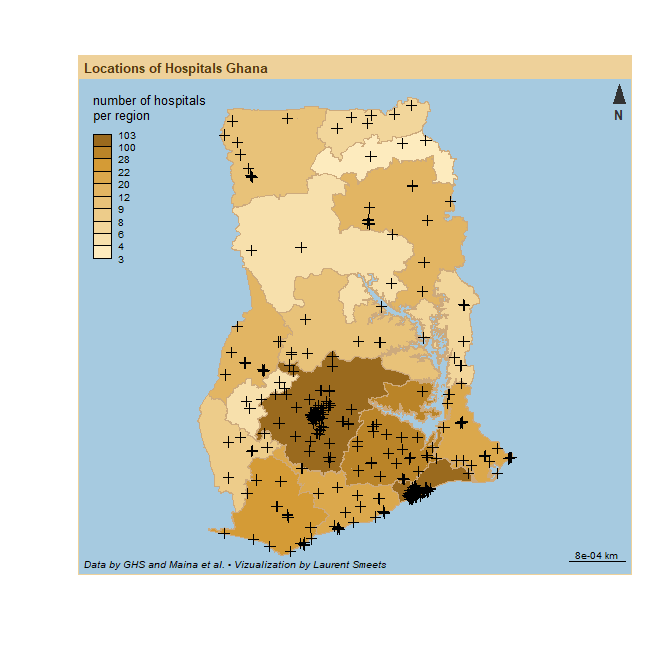
Now I have 369 hospitals with name and location. As a first step I can plot these on an overlay of the map of Ghana. In 2019, Ghana went from 10 to 16 regions, so most data and shapefiles that are available online still use the 10 region. I found a shape file of the 16 regions here.
# load the shape file both as sf and  SpatialPolygonsDataFrame
Ghana_16_region <- st_read("GHANA_16_REGIONS-shp/GHANA_16_REGIONS.shp",   quiet = TRUE)
Ghana_16_region_df <- rgdal::readOGR("GHANA_16_REGIONS-shp/GHANA_16_REGIONS.shp", layer= "GHANA_16_REGIONS", verbose=FALSE)
Ghana_16_region <- select(Ghana_16_region, REGION, Shape__Are )

# set the hospital as SpatialPointsDataFrame
coordinates(dat_complete) <- ~ Longitude + Latitude
proj4string(dat_complete) <- proj4string(Ghana_16_region_df)

# using the over() function  to check in which of the 16 regions a hospital is located
dat_complete_df <-  bind_cols(as_tibble(dat_complete),
                                sp::over(dat_complete, Ghana_16_region_df, fun = "sum"))

# summarize the number of hospitals per region
Ghana_16_region <- Ghana_16_region %>%
  left_join(
  dat_complete_df %>%
  group_by(REGION ) %>%
  summarise(N_hospitals = n()),
  by = "REGION")

# create colour breaks
bks <- getBreaks(v = Ghana_16_region$N_hospitals, method = "jenks", nclass = 10)
cols <- carto.pal(pal1 = "sand.pal", n1 = 11)

# plot the background
plot(Ghana_16_region$geometry, border = NA, col = NA, bg = "#A6CAE0")

# plot a choropleth with number of hospitals per region
choroLayer(
  add = TRUE,
  x = Ghana_16_region,
  var = "N_hospitals",
  breaks = bks,
  border = "burlywood3",
  col = cols,
  legend.pos = "topleft",
  legend.values.rnd = 1,
  legend.title.txt = "number of hospitals\nper region"
)
# plot the hospital points
plot(dat_complete, add = T)

# add labels
layoutLayer(title = "Locations of Hospitals Ghana",
            author = "Data by GHS and Maina et al. • Vizualization by Laurent Smeets",
            frame = TRUE,
            scale = "auto",
            north = TRUE,
            theme = "sand.pal")
Driving Times
To calculate this driving times, I need to query some type of routing service to calculate the driving distance (or driving actually time) from a given place to the nearest hospital Google Maps would be one option to use, but that is not a free API to use, so the Open Source Routing Machine (OSRM) is a more suitable open-source alternative. There is an online demo version available, but that one will not be sufficient for the number of driving distances I want to calculate.
OSRM
To run OSRM on a windows machine, you would ideally have Docker Desktop installed (https://www.docker.com/products/docker-desktop). To do so you will need a newer version of Windows 10 (version 2004 or higher, released in May 2020). Install instructions can be found here.
After installing Docker desktop, you should also make sure you have the wget command installed for windows (if you are using a Windows operating system), more information on that
here. Now just open the Docker Desktop programme and your command line interface (type “CMD” into you Windows search bar to open the command line interface).
docker pull osrm/osrm-backend
Second navigate to the folder from where you want to run this project, by using the cd command.
cd NAME_OF_FOLDER\NAME_OF_SUBFOLDER\ETC
Then download the map of the country you want to use in this case Ghana.
wget http://download.geofabrik.de/africa/ghana-latest.osm.pbf
Now extract the data from this file (These commands are Windows specific for, Linux specific commands see the OSRM
tutorial page). As, I am interested in driving times I use opt/car.lua instead of opt/foot.lua.
#docker run -t -v %cd%:/data osrm/osrm-backend osrm-extract -p /opt/foot.lua /data/ghana-latest.osm.pbf
docker run -t -v %cd%:/data osrm/osrm-backend osrm-extract -p /opt/car.lua /data/ghana-latest.osm.pbf
It will end with something looking like this:
[info] ok, after 15.887s
[info] Processed 2214859 edges
[info] Expansion: 103744 nodes/sec and 31209 edges/sec
[info] To prepare the data for routing, run: ./osrm-contract "/data/ghana-latest.osrm"
[info] RAM: peak bytes used: 1406402560
Now you have to partition the data using this command:
docker run -t -v %cd%:/data osrm/osrm-backend osrm-partition /data/ghana-latest.osrm
Which will give you an output similar to this:
[info] Level 1 #cells 4479 #boundary nodes 102100, sources: avg. 15, destinations: avg. 22, entries: 1923670 (15389360 bytes)
[info] Level 2 #cells 370 #boundary nodes 14768, sources: avg. 26, destinations: avg. 39, entries: 492861 (3942888 bytes)
[info] Level 3 #cells 23 #boundary nodes 1300, sources: avg. 37, destinations: avg. 54, entries: 60780 (486240 bytes)
[info] Level 4 #cells 1 #boundary nodes 0, sources: avg. 0, destinations: avg. 0, entries: 0 (0 bytes)
[info] Bisection took 13.7743 seconds.
[info] RAM: peak bytes used: 487546880
Now you have to customize the data using this command:
docker run -t -v %cd%:/data osrm/osrm-backend osrm-customize /data/ghana-latest.osrm
Which will give you an output similar to this:
[info] MLD customization writing took 0.421035 seconds
[info] Graph writing took 0.503969 seconds
[info] RAM: peak bytes used: 400687104
Now you are ready to use OSRM, to start the programme simply run:
docker run -t -i -p 5000:5000 -v %cd%:/data osrm/osrm-backend osrm-routed --algorithm mld --max-table-size 10000 /data/ghana-latest.osrm
Which will give you an output similar to this:
[info] starting up engines, v5.22.0
[info] Threads: 8
[info] IP address: 0.0.0.0
[info] IP port: 5000
[info] http 1.1 compression handled by zlib version 1.2.8
[info] Listening on: 0.0.0.0:5000
[info] running and waiting for requests
options(osrm.server = "http://localhost:5000/", osrm.profile = "drving")
Building a Grid
I have the locations of the hospitals in Ghana, the next step is getting a grid of coordinates from where to calculate distances from. I could just draw a random sample of coordinates that lie within Ghana and calculate the driving time (in minutes) from these points to the nearest hospital, but it is more efficient to create a grid of coordinates. This means that every 0.025 degree in longitude and 0.025 degree in latitude within the bounding box of Ghana a coordinate is created. (I know that one degree difference in longitude is not the same a one degree difference in latitude in km. However, Ghana is close enough to zero degrees latitude and longitude (0°N 0°E), that this difference does really not matter that much. Also I will interpolate the data later so any tiny gaps will be smoothed over.)
See this page on how driving speeds are calculated in OSRM. In summary, base driving speed is set at the maximum speed of a road penalty multipliers are added for different types of road surfaces and traffic situations. For example, corners have a multiplier of .75, meaning that driving speed of a place with a 50km/h speed limits in a corner is not 50km/h but, but $50\cdot0.75 = 37.5$ km/h.
# extract the bouding box
bounding_box <- Ghana_16_region_df@bbox

# create the grid, using expand.grid()
grid <- expand.grid(seq(bounding_box[1,1], bounding_box[1,2], by = 0.025),
                    seq(bounding_box[2,1], bounding_box[2,2], by = 0.025)) %>%
  as_tibble() %>%
  mutate(id = 1:n()) %>%
  relocate(id) %>%
  setNames(c("id", "lon","lat"))


# plot the grid, with as background the shapefile of Ghana
ggplot() +
  geom_point(data = grid,
             aes(x = lon, y = lat),
             col = "red", size = .01) +
    geom_polygon(data = fortify(Ghana_16_region_df),
               aes(x=long, y=lat, group = group),
               fill = NA, col = "black") +
  theme_minimal()+
  coord_map()
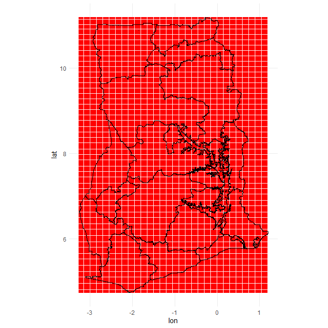
nrow(grid)
## [1] 46182
There are 46182 different points in this bounding box, but not all fall within the borders of Ghana To subset only those points that fall within Ghana I use the following code, using the over() command from the sp package.
coordinates(grid) <- ~ lon + lat
proj4string(grid) <- proj4string(Ghana_16_region_df)

# select only those points that lie within the country boundaries
points_in_polygon <- bind_cols(over(grid, Ghana_16_region_df) %>% select(REGION),
                               as_tibble(grid) %>% select(id, lon, lat )) %>%
  filter(!is.na(REGION )) %>%
  as_tibble() %>%
  select(-REGION ) %>%
  mutate(id = 1:n())

# plot it again
ggplot() +
  geom_point(data = points_in_polygon,
             aes(x = lon, y = lat),
             col = "red", size = .01) +
  geom_polygon(data = fortify(Ghana_16_region_df),
               aes(x=long, y=lat, group = group),
               fill = NA, col = "black") +
  theme_minimal()+
  coord_map()
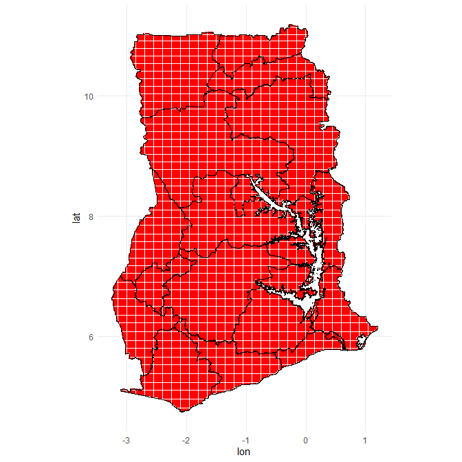
nrow(points_in_polygon)
## [1] 30343
Now there are only 30343 point left. The next part of code will take some time to run as it needs to calculate the traveling distance/time from 46182 locations to 369 hospitals (11,196,567 routes in total), and pick the shortest travel time. There are definitely ways to optimize this code (for example, I could decide to only calculate the route to the 10 Great-circle distance nearest hospitals and calculate travel times form them). But I only intend to run this code once, and computers are patient workers. I do split the points in some different sections, to limit the complexity on the OSRM server a bit. All in all, this takes like 5 minutes on my machine.
# Split data in to chunks of 500
points_in_polygon$section <- rep(1:ceiling(nrow(points_in_polygon)/500), each = 500)[1:nrow(points_in_polygon)]

# this input to the osrmTable is only allowed to have 3 columns.
hospital_locations_lat_long <- dat_complete_df %>%
  mutate(id = 1:n()) %>%
  select(id, Longitude, Latitude) %>%
  rename(lat = Latitude,
         lon = Longitude)

# create an empty list
list_points <- list()

# iterate of the different 500 point chunks
for(i in unique(points_in_polygon$section)){

  # select current chunk
  data_points <- points_in_polygon %>%
  filter(section == i) %>%
  select(-section)

  # this is the OSRM function that calculates the travel time
  travel_time_story <- osrmTable(src = data_points,
                                 dst = hospital_locations_lat_long,
                                 measure = "duration")

  # for every point the function calculates the travel time to every hospital
  # I only need to save the driving duration to the nearest hospital
  list_points[[i]] <- bind_cols(travel_time_story$sources,
                                 mintime = apply(travel_time_story$durations, 1, min)) %>%
    as_tibble()

}

# I  bind the travel duration back on to the original grid
points_in_polygon_with_travel_times <- data.table::rbindlist(list_points) %>%
  bind_cols(points_in_polygon %>%
              select(lon, lat) %>%
              rename(lon.org = lon,
                     lat.org = lat))
median(points_in_polygon_with_travel_times$mintime)
## [1] 39.9
mean(points_in_polygon_with_travel_times$mintime)
## [1] 48.09315
The median travel time from any given point in Ghana is around 40 minutes and the mean travel time 48 minutes (that does of course not mean that the average Ghanaian lives 40 minutes from a hospital, as this does not take population density into consideration).
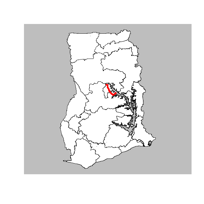
We can also calculate the longest possible travel time to the nearest hospital.
longest_travel_time <- points_in_polygon_with_travel_times[which.max(points_in_polygon_with_travel_times$mintime), ]

longest_travel <- osrmTable(src = data.frame(id = 1 ,
                          lon = longest_travel_time[1,4],
                          lat = longest_travel_time[1,5]),
          dst = hospital_locations_lat_long,
          measure = "duration")


longest_travel_df <- tibble(id = 1,
                            longest_travel$sources[1],
       longest_travel$sources[2],
       mintime = apply(longest_travel$durations, 1, min),
       lon_end = longest_travel$destinations[which.min(longest_travel$durations), 1],
       lat_end = longest_travel$destinations[which.min(longest_travel$durations), 2])

route <- osrmRoute(src = longest_travel_df[,c(1,2,3)],
          dst = longest_travel_df[,c(1,5,6)],
          overview = "full",
          returnclass = "sf")
This route is around 3 hours and 20 minutes (according to OSRM algorithm over unpaved road) and the distance 94 km over
sub(":\\d{2}", "", times((route$duration%/%60 + route$duration%%60/3600)/24))
## [1] "03:18"
route$distance
## [1] 93.8869
If I quickly plan this road we see that it route is in Brong-Ahafo Region in the centre of Ghana.
# Display the path
plot(Ghana_16_region$geometry, border = "black", col = "white", bg = "grey")
plot(st_geometry(route), lwd = 5, add = TRUE, col = "red")
A bit more zoomed in the plot looks like this (using OpenStreetMap as a background).
osm <- getTiles(x = route, crop = FALSE, type = "osm", zoom = 13)
tilesLayer(osm)
plot(st_geometry(route), lwd = 4, add = TRUE)
plot(st_geometry(route), lwd = 1, col = "white", add = TRUE)
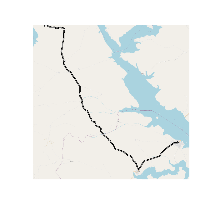
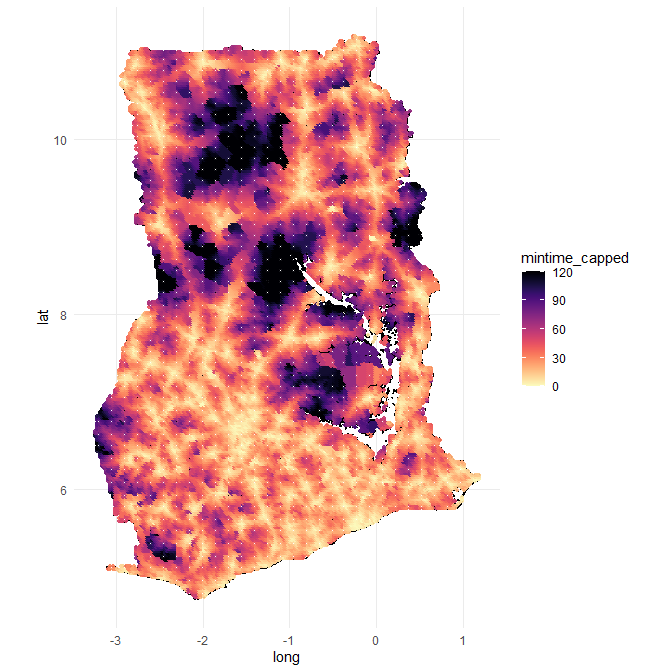
If I plot this, this is how it looks, It starts resembling what I am looking for.
# for points with more than 2 hour driving distance, I cap them at 2 hours (for plotting purposes)

points_in_polygon_with_travel_times <- points_in_polygon_with_travel_times %>%
    mutate(mintime_capped = ifelse(mintime > 120, 120, mintime))


ggplot() +
  geom_polygon(data = fortify(Ghana_16_region_df),
               aes(x=long, y=lat, group = group),
               fill = NA, col = "black") +
  geom_point(data = points_in_polygon_with_travel_times,
             aes(x = lon.org, y = lat.org, col = mintime_capped), size = .9, alpha = .9) +
               viridis::scale_color_viridis(option = "magma", direction = -1) +
  theme_minimal()+
  coord_map()
Beautify the Plot
Now we just need to make a raster file out of these points, interpolate between points, project it over a real map of Ghana, and make the plot a bit more beautiful.
##correct spatial reference for Ghana here: https://spatialreference.org/ref/
CRS_string <- "+proj=aea +lat_1=20 +lat_2=-23 +lat_0=0 +lon_0=25 +x_0=0 +y_0=0 +ellps=WGS84 +datum=WGS84 +units=m +no_defs"


# we set a resolution
gridRes  <- 100

# transform data to SpatialPointsDataFrame  with longitude/latitude projection
data_sp <- points_in_polygon_with_travel_times
coordinates(data_sp) <- ~lon.org+lat.org
proj4string(data_sp) <- crs("+init=epsg:4326")
coords <- c("lon", "lat")

data_sf <- st_as_sf(data_sp, coords = coords, crs = proj4string(data_sp))

# Reset it to the projection of Ghana
data_sp_mp <- spTransform(data_sp, CRSobj = CRS_string)


# Here we set the bounding box I want to use (plus a bit of a margin)
# We also create a new grid that is used for the interpolation

boxx = data_sp_mp@bbox
deltaX = as.integer((boxx[1,2] - boxx[1,1]) + 1.5)
deltaY = as.integer((boxx[2,2] - boxx[2,1]) + 1.5)
gridSizeX = deltaX / gridRes
gridSizeY = deltaY / gridRes
grd = GridTopology(boxx[,1], c(gridRes,gridRes), c(gridSizeX,gridSizeY))
pts = SpatialPoints(coordinates(grd))


# Reset it to the projection of Ghana
proj4string(pts) <- crs(CRS_string)

# create an empty raster
r.raster <- raster::raster()
# set the extent of the raster to the data points we gave
extent(r.raster) <- extent(pts)
# set the resolution (cell size)
res(r.raster) <- gridRes
# set the correct crs
crs(r.raster) <- crs(CRS_string) #

# Interpolate the grid cells Nearest neighbour function (k = 30) using the gstat package
gs <- gstat(formula = mintime_capped~1,
            locations = data_sp_mp,
            nmax = 30,
            set = list(idp = 0))

# This might take a while to run
raster_object <- interpolate(r.raster, gs)

# ad both object to a list
minraster <- list(data_sf, raster_object)
names(minraster) <- c("data", "raster_object")

# Instead of the 16 different regions, I can create a single shapefile of Ghana,
# combining all the regions into one shape file
Ghana_country <- as(st_union(Ghana_16_region), "Spatial")


Ghana_country <- spTransform(Ghana_country, CRSobj = CRS_string)
minraster_shaped <- mask(minraster$raster_object, Ghana_country)
#saveRDS(minraster_shaped , "minraster_shaped_120.RDS")
#saveRDS(CRS_string , "CRS_string.RDS")

CRS_string <- readRDS("CRS_string.RDS")
minraster_shaped <- readRDS("minraster_shaped_120.RDS")
To plot this is ggplot2 I need to make a polygon object out of the raster object.
# you could use this code to speed up the plotting.

 minraster_shaped_aggr <- aggregate(minraster_shaped, fact = 5)
# again, this function might take a while to run
# if it takes to long, set a higher aggregation factor
# or a higher Gridres
# or less points


minraster_shaped_rtp <- rasterToPolygons(minraster_shaped_aggr)

# we go back to standard long/lat projection for plotting purposes
minraster_shaped_rtp <- spTransform(minraster_shaped_rtp,
                                    CRS("+proj=longlat +datum=WGS84 +no_defs +ellps=WGS84 +towgs84=0,0,0"))

# Now I fortify this data to plot it
minraster_shaped_rtp@data$id <- 1:nrow(minraster_shaped_rtp@data)
minraster_shaped_fort <- fortify(minraster_shaped_rtp,
                                 data = minraster_shaped_rtp@data)
minraster_shaped_fort <- merge(minraster_shaped_fort,
                               minraster_shaped_rtp@data,
                               by.x = 'id',
                               by.y = 'id')
I would like to have some real map as a background, so I download it from Stamenmap and use a function I found here to crop out a polygon and plot the result.
# download background map tiles
# for this level of zoom, you might have to run this command a few times

Ghana_map_bg <- get_stamenmap(bbox = bounding_box, zoom = 9, maptype="terrain-background", color = "bw", crop = F)

# load the function to make a raster file out of the tiles
ggmap_rast <- function(map){
  map_bbox <- attr(map, 'bb')
  .extent <- extent(as.numeric(map_bbox[c(2,4,1,3)]))
  my_map <- raster(.extent, nrow= nrow(map), ncol = ncol(map))
  rgb_cols <- setNames(as.data.frame(t(col2rgb(map))), c('red','green','blue'))
  red <- my_map
  values(red) <- rgb_cols[['red']]
  green <- my_map
  values(green) <- rgb_cols[['green']]
  blue <- my_map
  values(blue) <- rgb_cols[['blue']]
  stack(red,green,blue)
}


# make a raster file out of the maps
Ghana_map_bg_rast <- ggmap_rast(Ghana_map_bg)

# crop the raster file
Ghana_map_bg_rast_masked <- mask(Ghana_map_bg_rast, Ghana_16_region_df, inverse=F)

# create a geospatial dataframe out of the raster file
Ghana_map_crop_masked_df <- data.frame(rasterToPoints(Ghana_map_bg_rast_masked))

sysfonts::font_add_google("Cinzel", "Cinzel") # this is the font I will be using

#These are needed to render the fonts
showtext_auto()
x11()
# create the map in ggplot
static_map  <- ggplot() +
   geom_point(data = Ghana_map_crop_masked_df,
              aes(x = x,
                  y = y,
                  col = rgb(layer.1/255,
                            layer.2/255,
                            layer.3/255))) +
  geom_polygon(data = fortify(Ghana_16_region_df),
               aes(x=long, y=lat, group = group),
               fill = "grey", col = "black") +
  scale_color_identity() +
  geom_polygon(data = minraster_shaped_fort,
               aes(x = long,
                   y = lat,
                   group = group,
                   fill = var1.pred,
                   alpha = var1.pred),
               size = 0) +
  scale_fill_gradient(high = "darkred",
                       low = "white",
                       name = "Driving Time",
                       limits = c(0, 120),
                       breaks = c(0, 60, 120),
                       labels = c("0","1h", "+2h"),
                       guide = guide_colorbar(
                         direction = "horizontal",
                         barheight = unit(10, units = "mm"),
                         barwidth = unit(5, units = "inch"),
                         draw.ulim = T,
                         title.position = 'top',
                         title.hjust = 0.5,
                         label.hjust = 0.5,
                         legend.location = "bottom"))+
  scale_alpha_continuous(guide = "none",
                         range = c(0.5, .9))+
  geom_point(data = dat_complete_df, aes(x=Longitude   , y=Latitude ),
             col = "white",
             size = 2,
             shape = 16,
             alpha= .8)  +
  labs(title  = "Driving Time to Nearest Hospital",
       caption = "Data by OpenStreetMap • Map by Stamenmap • Driving times by OSRM • Visualization by Laurent Smeets") +
  coord_map()+
  theme_minimal()+
  theme(
    # Change plot and panel background
    legend.position = "bottom",
    plot.background=element_rect(fill = "black"),
    panel.background = element_rect(fill = 'black'),
    plot.title = element_markdown(family = "Cinzel",
                                  size = 70,
                                  face = "bold",
                                  hjust = 0.5,
                                  color = "white",
                                  margin = margin(t = 20, b = 2)),
    legend.title = element_markdown(family = "Cinzel",
                                    color = "white",
                                    size = 50
                                    ),
    legend.text = element_text(size = 50,
                               color = "white"),
    plot.caption = element_markdown(size = 25,
                                color = "white",
                                family = "Cinzel",
                                hjust = 0.5))


#Do not save this is a .PDF, the raster file as a polygon, is HUGE in a vector file format
ggsave("static_map_high_res.png", static_map, height = 12, width = 8, dpi = 300)
This is how the plot looks:
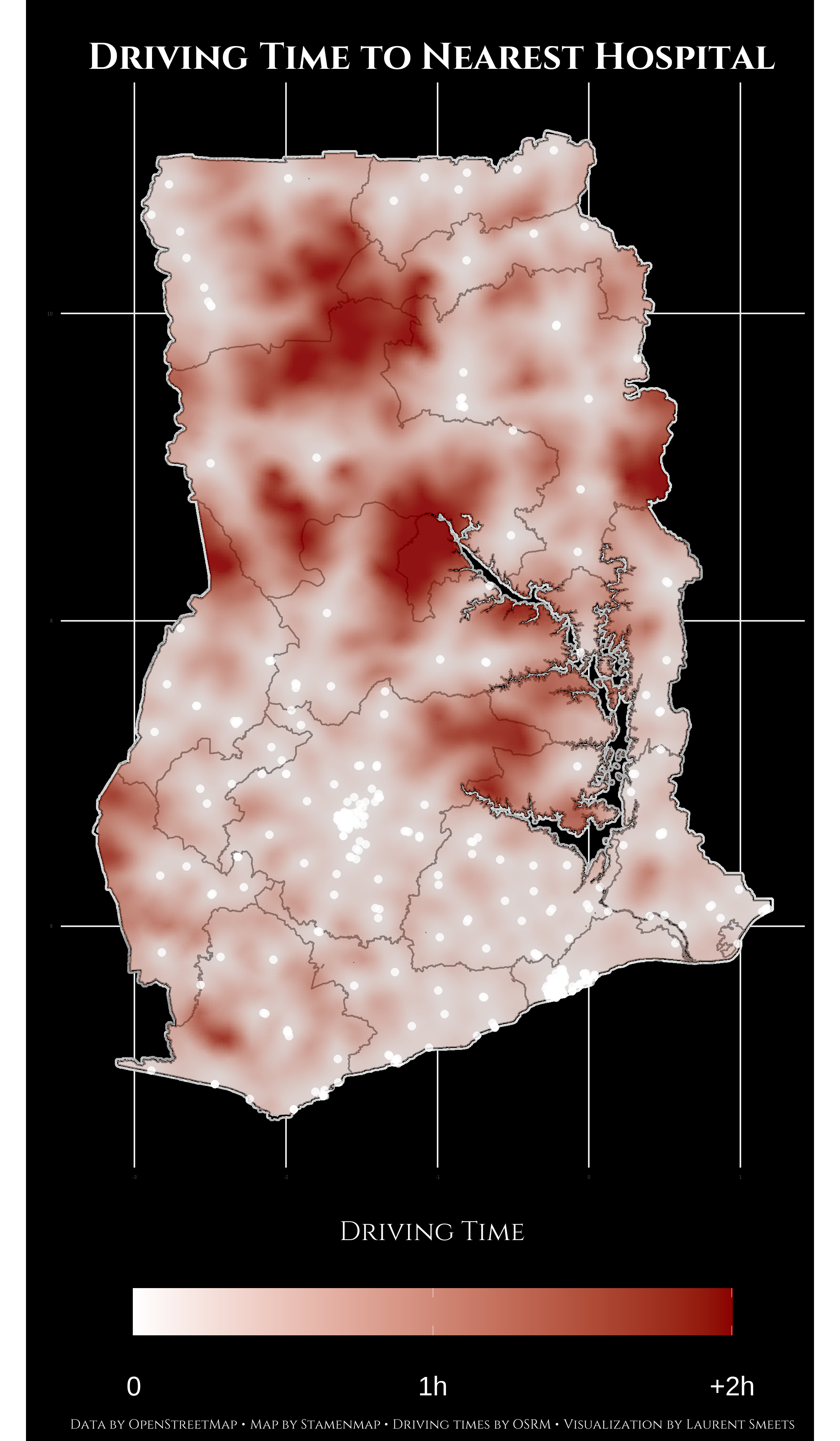
Notes on Map
- Please do not use this data in any form as medical (travel) advice. I have not verified the operation status of any of these hospital, nor am I familiar with the quality of medical service at any of these hospitals.
- The big red cloud of far travel times in the North East of the country correspond with the location of Mole National Park.
- In general, you can, as expected, see the furthest travel times outside of big cities and between major highways.
- This information does not take traffic into consideration. Anyone who has ever been in Accra can tell you that even within Accra you can travel 2 hours to the nearest hospital on a Friday afternoon.
Ghana Data Stuff
This website is my hobby project to showcase some of the project I am working one, when I am not working on the official statistics at the Ghana Statistical Service.