Plotting Street Name Suffixes in R
Introduction
In this document I will show how I created this nice map depicting the different suffixes of all the streets in Accra, Ghana. This requires loading data from
OpenStreetMap, cleaning these data, and some advance plotting in ggplot2. I will also make use of the new ggtext package to create some beautiful and colourful plot titles.
This code took heavy inspiration and some direct code from these sources, all credits to these original authors. Please have a look at what they did and some of the great tutorials they wrote:
- http://joshuamccrain.com/tutorials/maps/streets_tutorial.html
- https://github.com/Z3tt/30DayMapChallenge/tree/master/contributions/Day15_Names
- https://github.com/erdavis1/RoadColors
Packages
These are the packages used for this project:
library(sf)
library(foreign)
library(tidyverse)
library(osmdata)
library(ggtext)
library(showtext)
library(stringr)
# font_add_google("Oswald", "Oswald") # this is the font I will be using
Download raw data
I am using the osmdata package to download the data directly from OSM into R, but for this project you could also download the data to your machine first and then pull it in to R. You can find the relevant file (.shp.zip) for the whole of Ghana
here.
loc <- "Accra Ghana" # This is the city I want to create a map for

bounding_box <- getbb(loc) # this function looks for the square bounding box for this city

# I like to add a bit of margins to all sides of the bounding box
bounding_box_wide <- bounding_box
bounding_box_wide["x", "min"] <- bounding_box["x", "min"] - 0.1
bounding_box_wide["y", "min"] <- bounding_box["y", "min"] - 0.1
bounding_box_wide["x", "max"] <- bounding_box["x", "max"] + 0.1
bounding_box_wide["y", "max"] <- bounding_box["y", "max"] + 0.1
This what the boding box now looks likes
bounding_box_wide
##          min       max
## x -0.4657437 0.0542563
## y  5.3000141 5.8200141
Using this bounding box we can now download the data from OSM using the syntax of the osmdata package
roads <- bounding_box_wide %>%
  opq()%>%
  add_osm_feature(key = "highway") %>%
  osmdata_sf()

# Since we are plotting roads, we are just interested in the OSM lines
# We can omit things like OMS points and polygons
roads <- roads$osm_lines

# remove unnamed footpaths
roads <- roads[!(roads$highway  == "footway" & is.na(roads$name)),]
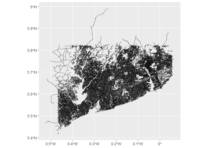
We can simply plot these roads like this:
ggplot() +
  geom_sf(data = roads,
          inherit.aes = FALSE,
          color = "black",
          size = .05,
          alpha = .5)
Subset Data
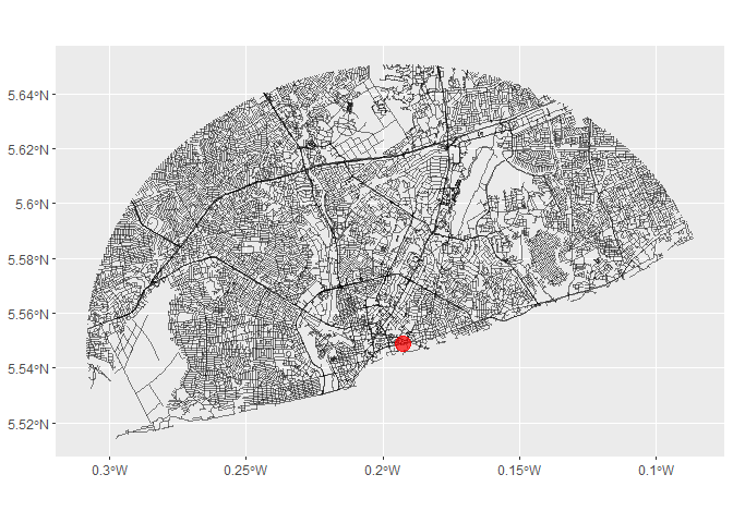
I personally think it is a nice visual effect to plot a circular city with a well-defined central point. Of course, no city’s boundaries are actually round and neither are those of Accra, this is just a visual effect. I just think it is a nice visual effect to centre Accra around a Independence square and the Black Star Gate, so I looked up the coordinates of the square and drew a 12km radius around it and filtered all road (segments) within that radius. To draw this circle I had to look up the correct spatial reference here: https://spatialreference.org/ref/. If you are using this code for a city that is not in West-Africa, you probably need to use a different reference system.
# subset the roads into a circle.
mid_point <- data.frame(lat = 5.548790, long = -0.192898 ) %>%  # This is the location of Black Star Gate
  st_as_sf(coords = c("long", "lat"), crs = 4326) %>% # # standardize the map projection
  st_transform("+proj=aea +lat_1=20 +lat_2=-23 +lat_0=0 +lon_0=25 +x_0=0 +y_0=0 +ellps=WGS84 +datum=WGS84 +units=m +no_defs ")

circle <- st_buffer(mid_point, dist = 12000) # this dist is distance in meters.
circle <- circle %>% st_transform(st_crs(roads))
roads <- st_intersection(circle, roads)
Now the map looks like this (With a red dot for the Black Star Gate)
ggplot() +
  geom_sf(data = roads,
          inherit.aes = FALSE,
          color = "black",
          size = .1,
          alpha = .5) +
  geom_sf(data = mid_point,
          inherit.aes = FALSE,
          color = "red",
          size = 5,
          alpha = .7)
Get Street Names
With some simple regex manipulations, using the stringr package, we can see what are common street suffixes in Accra (only within this 24km diameter). First lets see how the data looks like, by showing the first 20 road names.
roads$name[1:20]
##  [1] "Nortei Ababio Road"    NA                      NA
##  [4] "Volta Road"            "South Liberation Link" NA
##  [7] NA                      NA                      "4th Circular Road"
## [10] "John Churcher Loop"    NA                      NA
## [13] "Patrice Lumumba Road"  NA                      NA
## [16] "Jasmine Road"          "Prestige Link"         "2nd Circular Road"
## [19] "Kakramadu Road"        "Violet Road"
And this is how we can extract the suffixes for these roads
word(roads$name,-1)[1:20]
##  [1] "Road" NA     NA     "Road" "Link" NA     NA     NA     "Road" "Loop"
## [11] NA     NA     "Road" NA     NA     "Road" "Link" "Road" "Road" "Road"
Some content knowledge is needed to write code like this. For example, this code assumes that the street suffix comes after the main name of the street. So, in France where road names might start with Rue instead of end with it, this would not work. Similarly, in places like the Netherlands where the suffix is attached to the name (e.g. Dorpstraat), this would not work.
If we tabulate the results this is what we get these results:
table(stringr::word(roads$name,-1), exclude=NULL)
##
##                        10           18  Addo)street Agbogbloshie        Alley
##           27            5            1            1           10            4
##       Avenue      Avernue       Bonnie    Boulevard       Bridge     Broadway
##          555           12            1            5            1            2
##     Bulevard         Bush      Central        Circ.       Circle        close
##            2            1           78            1           51            1
##        Close        CLose        Court     crescent     Crescent      Cresent
##          301            1            1            5          117            1
##        Drive         East          Esi    Extension         Gate        Guava
##           62           15            2            9            3            1
##      Hermosa      Highway  Hypermarket  Interchange     Junction         Kubi
##            1          149            4           23            1            1
##       Lagoon         lane         Lane         LAne         link         Link
##            3            3          187            1            1          219
##        Linlk         Linx         Loop       Mawena       Mawuli       Mirada
##            1            1           45            2            1            1
##       Mosque     Motorway        Ofram      Ollennu         Oyeo         path
##            1           82            1            2           11            1
##         Path     proposed         Raod        Ridge         road         Road
##            2            1            9            3           20         1172
##          Rod   Roundabout     Shortcut      Sithole          Sol        South
##            1           60            1            4            1            1
##        Spiga           St       Streer       street       Street        Stret
##            1            1            1            7         1396            1
##       Tunnel        Vista        Volta         Walk          Way         West
##            1            4            2            2           13           14
##         <NA>
##        10905
Data Cleaning
We see that there are quite some missing values (meaning that street is not named), and quite some misspellings. Surely “Avernue”, should just be “Avenue”. I need to clean this data first, before I can plot it. These are the steps I took:
- fix certain common misspelling
- For roads that have as suffix a cardinal direction (Ring Road East, Ring Road West, etc.) do not look at the last word of the street name, but the second to last word
- If the name street name is missing, simply call it “Unnamed’
- At this stage I am going to concatenate “Highways” and “Motorways” into one category instead of two categories
misspellings <- tribble(
  ~org, ~target,
  "10",   "Unnamed",
  "1", "Unnamed",
  "18", "Unnamed",
  "avenue",   "Avenue",
  "Avernue",   "Avenue",
  "Bulevard",   "Boulevard",
  "Circ.", "Circle",
  "close", "Close",
  "CLose", "Close",
  "Cresent ", "Crescent",
  "crescent", "Crescent",
  "lane", "Lane",
  "LAne", "Lane",
  "Linlk", "Link",
  "Lk", "Link",
  "LK", "Link",
  "Linx", "Link",
  "Raod", "Road",
  "road", "Road",
  "Rod", "Road",
  "Rd", "Road",
  "Rd.", "Road",
  "Roaf", "Road",
  "LP", "Loop",
  "Addo)street",   "Street",
  "St", "Street",
  "Streer", "Street",
  "street", "Street",
  "Stret", "Street")


roads_cleaned <- roads %>%
  mutate(Suffix = ifelse(is.na(name), "Unnamed",
                         ifelse(tolower(stringr::word(name,-1)) %in% c("north", "west", "east", "south", "central"),
                                stringr::word(name,-2),
                                stringr::word(name,-1)))) %>%
  left_join(misspellings, by = c("Suffix" = "org")) %>%
  mutate(Suffix = ifelse(is.na(target), Suffix, target),
         Suffix = ifelse(Suffix %in% c("Motorway", "Highway"), "Motorway/Highway", Suffix)) %>%
  select(osm_id, highway, name,  Suffix, geometry)
Common suffixes
Lets see what the most common road suffixes are in Accra.
top_road_names <- roads_cleaned %>%
  select(Suffix) %>%
  as_tibble() %>%
  count(Suffix) %>%
  arrange(desc(n)) %>%
  top_n(11, n)

top_road_names
## # A tibble: 11 x 2
##    Suffix               n
##    <chr>            <int>
##  1 Unnamed          10911
##  2 Street            1407
##  3 Road              1309
##  4 Avenue             567
##  5 Close              303
##  6 Motorway/Highway   231
##  7 Link               222
##  8 Lane               191
##  9 Crescent           122
## 10 Drive               62
## 11 Roundabout          60
Percentage of Roads with Suffix
There are two ways to calculate the prevalence of road suffixes, either by total roads with a given suffix or by km of road with a given suffix. This first option is not ideal, since OSM data splits a road in many different segments and maybe there is some bias on how this happens. Maybe straight lines highways are split in less segments than unnamed curvy backroads, or vice versa. So it is better to base calculation on the total of km of roads with a certain suffix. To calculate the lengths of roads we can use the st_length() function. I also did some further data cleaning and renamed all suffixes that are not among the 11 most common names to “Other”.
roads_cleaned <- roads_cleaned %>%
  mutate(length_road = st_length(geometry)) %>%
  mutate(Suffix = ifelse(Suffix %in% c(top_road_names$Suffix), Suffix, "Other"))
Now I can summarise these results.
summary_stats <- roads_cleaned %>%
  select(-geometry) %>%
  as_tibble() %>%
  group_by(Suffix) %>%
  summarise(km = as.numeric(sum(length_road)/1000),
            n = n(),
            mean_km = km/n,
            .groups = "drop") %>%
  mutate(percent_road_network = km/sum(km),
         percent_roads = n/sum(n))
This is how this looks in a bar chart:
summary_stats %>%
  ggplot() +
  geom_bar(aes(x = reorder(Suffix,percent_road_network) ,
               y = percent_road_network), stat = "identity") +
  scale_y_continuous(labels = scales::percent_format()) +
  coord_flip()
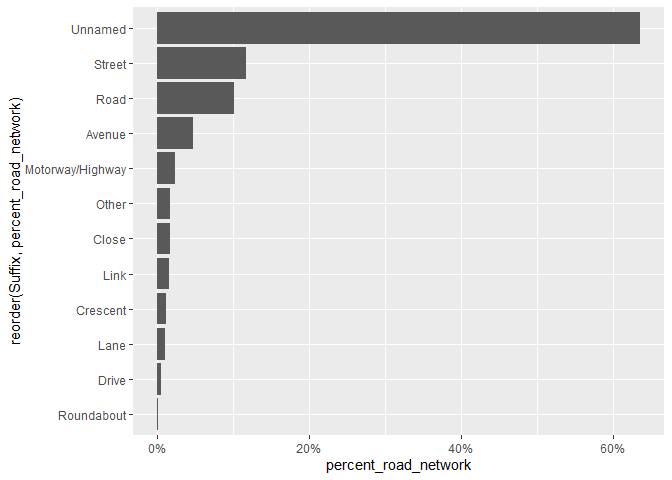
Around 63.3% of roads are still unnamed in Accra, Ghana (well, at least on OSM).
Extra Data Manipulations
Some final data manipulations are in order to make this map look like a proper map. For example, I downloaded the railways and bodies of water (rivers, streams and canals) from OSM to make the map extra ‘map-like’.
# Download rivers
rivers <- st_bbox(roads_cleaned) %>%
  opq()%>%
  add_osm_feature(key = "waterway", value = c("river", "canal", "stream")) %>%
  osmdata_sf()

rivers <- rivers$osm_lines
rivers <- st_transform(rivers,st_crs(roads_cleaned))
rivers <- st_intersection(circle, rivers)

# Download railways
railways <- st_bbox(roads_cleaned)%>%
  opq()%>%
  add_osm_feature(key = "railway", value="rail") %>%
  osmdata_sf()

railways <- railways$osm_lines
railways <- st_transform(railways,st_crs(roads_cleaned))
railways <- st_intersection(circle, railways)
I also want t0 specify the thickness of different roads, so that, for example, Motorways are plotted thicker than normal residential roads
roads_cleaned <- roads_cleaned %>%
  mutate(Suffix = ifelse(Suffix %in% c(top_road_names$Suffix), Suffix, "Other")) %>%
  mutate(road_type = ifelse(highway %in% c("motorway",
                                          "primary",
                                          "motorway_link",
                                          "primary_link"),
                            "fat",
                            ifelse(highway %in% c("secondary",
                                                 "tertiary",
                                                 "secondary_link",
                                                 "tertiary_link"),
                                   "medium",
                                   "thin")))
Now I add the percentage of road suffixes to the legend.
labels_colors  <- summary_stats %>%
  mutate(percent_road_network  = as.numeric(percent_road_network) *100) %>%
  mutate(label = paste0(Suffix, " (", round(percent_road_network, 1), "%)")) %>%
  select(label) %>%
  unlist(use.names = FALSE)

names(labels_colors) <- summary_stats$Suffix
I also assign different colours to the different types of streets and I manually set the order of the legend (mostly to guarantee that ‘Other’ and ‘Unnamed’ are the two last categories in the legend).
street_colours <- c("Unnamed" = "#c6c6c6",
                    "Street" = "#193264FF",
                    "Close" = "#B8A463",
                    "Avenue" = "#434C5E",
                    "Crescent" = "#F46D43",
                    "Drive"= "#651eac",
                    "Motorway/Highway" = "#E6F598",
                    "Lane" = "#CC6666",
                    "Link" = "#FDDBC7",
                    "Other" = "#B48EAD",
                    "Road" = "#9E0142",
                    "Roundabout" = "#66C2A5")

order <- c("Street",
           "Road",
           "Avenue",
           "Motorway/Highway",
           "Close",
           "Link",
           "Crescent",
           "Lane",
           "Drive",
           "Roundabout",
           "Other",
           "Unnamed")
# some re-ordering is needed to make use that the unnamed layers are
# plotted below the order layers

plot <- roads_cleaned %>%
  mutate(Suffix = factor(Suffix, levels = c("Unnamed",
                                            "Link",
                                            "Drive",
                                            "Other",
                                            "Avenue",
                                            "Close",
                                            "Street",
                                            "Lane",
                                            "Crescent",
                                            "Road",
                                            "Motorway/Highway",
                                            "Roundabout"))) %>%
  ggplot() +
  geom_sf(data = rivers,
          color = "steelblue",
          size = .9,
          alpha = .6) +
  geom_sf(data = railways,
          inherit.aes = FALSE,
          color = "black",
          size = 1,
          linetype = "dotdash",
          alpha = 1)+
  geom_sf(aes(colour = Suffix,
              size = road_type),
          alpha = 1,
          show.legend = "point") +
  scale_color_manual(values = street_colours,
                    labels = labels_colors,
                    breaks = order)+
  scale_size_manual(values = c(2, 1, .3)) +
  theme_void() +
  theme(  panel.background = element_rect(fill = "white",  #"grey92" would also look good
                                          color = "white"),
          plot.background = element_rect(fill = "white",
                                         color = "grey60",
                                         size = 7 ),
          plot.margin =  margin(20, 30, 20, 30),
          plot.title = element_markdown(family = "Oswald",
                                        size = 54,
                                        face = "bold",
                                        hjust = 0.5,
                                        margin = margin(t = 20, b = 2)),
          legend.position = "top",
          legend.box.spacing = unit(0.2, "cm"),
          legend.key = element_rect(fill = NA, color = NA),
          legend.key.size = unit(1, "lines"),
          legend.text = element_text(family = "Oswald",
                                     color = "grey60",
                                     size = 12,
                                     face = "bold"))  +
  guides(color = guide_legend(title.position = "top",
                              title.hjust = 0.5,
                              nrow = 2,
                              label.position = "right",
                              override.aes = list(size = 7.5))) +
  guides(size = F) +
  # The colours of the Titles are based on the colour codes of the Ghanaian flag,
  # which can be found here: https://www.schemecolor.com/ghana-flag-colors.php
  labs(title = "<b style='color:#CE1126'>STREET <b style='color:#FCD116'>NAMES</b><b style='color:#000000'> OF</b><b style='color:#006B3F'> ACCRA</b>",
       fill  = NULL,
       col  = NULL) +
  annotate("text",
           x = mean(c(st_bbox(roads_cleaned$geometry)["xmin"],
                      st_bbox(roads_cleaned$geometry)["xmax"])), # to centre it
           y = 5.515,
           hjust = 0.5,
           vjust = 1,
           label = "    Visualization by Laurent Smeets  •   Data from OpenStreetMap", # some extra spaces to align the • in the centre
           family = "Oswald",                                                          # One day I will find a better solution
           size = 4.5,
           color = "grey60")
save plot in high-res
ggsave("plot_accra_streets2.png", plot, height = 11, width = 15, dpi = 1000)
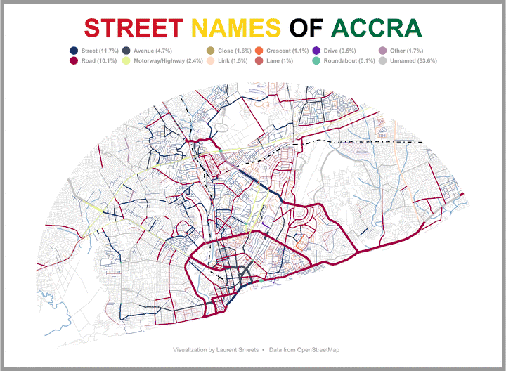
This is how the final plot looks.
Ghana Data Stuff
This website is my hobby project to showcase some of the project I am working one, when I am not working on the official statistics at the Ghana Statistical Service.