Plotting the Average Walking Distance to the Nearest Bar in Accra

Introduction
What is the best place to live in Accra, or any other city for that matter? Well clearly a neighbourhood with plenty of bars available or at least a bar within a short walking distance. This is a little experiment for me to try to plot a walking distance heatmap to a nearest bar in R. This involves getting data from OSM, planning walking routes and times is OSRM, plotting in leaflet and ggplot2, using the sp, sf, raster, jstat, osmdata, and osrm packages.
This code took heavy inspiration and some direct code from these sources, all credit to these authors. Please have a look at what they did and some of the great tutorials they wrote:
- https://rcarto.github.io/caRtosm/index.html
- https://mtmx.github.io/blog/bistrographie/
- https://dieghernan.github.io/cartographyvignette/
- https://rpubs.com/mgei/drivingtimes
- https://www.user2019.fr/static/pres/lt257361.pdf
Packages
These are the packages used for this project:
library(tidyverse)
library(osmdata)
library(sf)
library(spatstat)
library(maptools)
library(raster)
library(RColorBrewer)
library(leaflet)
library(sp)
library(gstat)
library(osrm)
library(ggmap)
library(ggtext)
library(cartography)
library(showtext)

# The raster package overrides the dplyr select function, so assign I assigned it back
select <- dplyr::select
loc <- "Accra Ghana" # This is the city I want to create a map for.
bounding_box <- getbb(loc) # this function looks for the square bounding box for this city.

accra_boundries <-bounding_box %>%
  opq() %>%
  add_osm_feature(key = 'name', value= "Accra Metropolitan") %>%
  osmdata_sp()

accra_boundries <- accra_boundries$osm_multipolygons[1,]
Using the available_tags('amenity') command we can see what types of different amenities OSM distinguishes.
available_tags('amenity')
##   [1] "animal_boarding"               "animal_shelter"
##   [3] "arts_centre"                   "atm"
##   [5] "baby_hatch"                    "baking_oven"
##   [7] "bank"                          "bar"
##   [9] "bbq"                           "bench"
##  [11] "bicycle_parking"               "bicycle_rental"
##  [13] "bicycle_repair_station"        "biergarten"
##  [15] "boat_rental"                   "boat_sharing"
##  [17] "brothel"                       "bureau_de_change"
##  [19] "bus_station"                   "cafe"
##  [21] "car_rental"                    "car_sharing"
##  [23] "car_wash"                      "casino"
##  [25] "charging_station"              "childcare"
##  [27] "cinema"                        "clinic"
##  [29] "clock"                         "college"
##  [31] "community_centre"              "conference_centre"
##  [33] "courthouse"                    "crematorium"
##  [35] "dentist"                       "dive_centre"
##  [37] "doctors"                       "drinking_water"
##  [39] "driving_school"                "embassy"
##  [41] "fast_food"                     "ferry_terminal"
##  [43] "fire_station"                  "firepit&action=edit&redlink=1"
##  [45] "food_court"                    "fountain"
##  [47] "fuel"                          "gambling"
##  [49] "give_box"                      "grave_yard"
##  [51] "grit_bin"                      "gym"
##  [53] "hospital"                      "hunting_stand"
##  [55] "ice_cream"                     "internet_cafe"
##  [57] "kindergarten"                  "kitchen"
##  [59] "kneipp_water_cure"             "language_school"
##  [61] "library"                       "marketplace"
##  [63] "monastery"                     "motorcycle_parking"
##  [65] "music_school"                  "nightclub"
##  [67] "nursing_home"                  "parking"
##  [69] "parking_entrance"              "parking_space"
##  [71] "pharmacy"                      "photo_booth"
##  [73] "place_of_worship"              "planetarium"
##  [75] "police"                        "post_box"
##  [77] "post_depot"                    "post_office"
##  [79] "prison"                        "pub"
##  [81] "public_bath"                   "public_bookcase"
##  [83] "public_building"               "ranger_station"
##  [85] "recycling"                     "refugee_site"
##  [87] "restaurant"                    "sanitary_dump_station"
##  [89] "sauna"                         "school"
##  [91] "shelter"                       "shower"
##  [93] "social_centre"                 "social_facility"
##  [95] "stripclub"                     "studio"
##  [97] "swingerclub"                   "taxi"
##  [99] "telephone"                     "theatre"
## [101] "toilets"                       "townhall"
## [103] "toy_library"                   "university"
## [105] "vehicle_inspection"            "vending_machine"
## [107] "veterinary"                    "waste_basket"
## [109] "waste_disposal"                "waste_transfer_station"
## [111] "water_point"                   "watering_place"
For this project I will just pick “biergarten” (I do not think there are too many of these in Accra), “pub”, “bar” and “nightclub.”
# select the relevant amenities
bars_accra <- st_bbox(accra_boundries) %>%
  opq() %>%
  add_osm_feature(key = 'amenity',
                  value = c("biergarten", "pub", "bar", "nightclub")) %>%
  osmdata_sp()

# only select the location points
bar_locations <- bars_accra$osm_points %>%
  as_tibble() %>%
  select( osm_id,  name, lon, lat )

# subset only those points that fall within the city boundaries of Accra
accra_boundries <- sp::spTransform(accra_boundries, CRS("+proj=longlat"))

coordinates(bar_locations) <- ~ lon + lat
proj4string(bar_locations) <- proj4string(accra_boundries)

bars_accra_data_frame <- bind_cols(over(bar_locations, accra_boundries) %>% select(type),
                                   as_tibble(bar_locations) %>% select(osm_id, name, lon, lat )) %>%
  filter(!is.na(type)) %>%
  as_tibble() %>%
  mutate(across(where(is.factor), ~as.character(.))) %>%
  select(-type)
Lets see the first 5 results:
bars_accra_data_frame %>% head(5)
## # A tibble: 5 x 4
##   osm_id     name                        lon   lat
##   <chr>      <chr>                     <dbl> <dbl>
## 1 373239152  Epo's Spot               -0.185  5.56
## 2 1151761364 Bloom Bar                -0.180  5.56
## 3 1270558373 Boomerang                -0.217  5.58
## 4 1368374881 Roxbury                  -0.204  5.57
## 5 1616146876 The Honeysuckle - Labone -0.173  5.57
Density map of Bars
This some what of an overkill, one could just plot the bars as points in ggplot2 and use geom_density2d() to plot the kernel density. However, since I am working with geo-spatial points, this option offers a bit more flexibility and is just a bit better looking. This also means I can plot the resulting density estimation over a leaflet map, which allows me to hover over the bars to see their names.
# correct spatial reference for Ghana can be found here: https://spatialreference.org/ref/

CRS_string <- "+proj=aea +lat_1=20 +lat_2=-23 +lat_0=0 +lon_0=25 +x_0=0 +y_0=0 +ellps=WGS84 +datum=WGS84 +units=m +no_defs"

# change from sp to st object and change the projection reference
accra_boundries_st <- st_transform(st_as_sf(accra_boundries), CRS_string)

# set the coordinates of the bars to the same reference
coordinates(bars_accra_data_frame) <- ~ lon + lat
proj4string(bars_accra_data_frame) <- proj4string(accra_boundries)
bar_locations_crs <- st_transform(st_as_sf(bars_accra_data_frame), CRS_string)

# Transform them in Spatial objects (SpatialPointsDataFrames)
bar_locations_spatial <- as(bar_locations_crs, "Spatial")
accra_boundries_spatial <- as.owin(as(accra_boundries_st, "Spatial"))

# extract just the coordinates of the bars
bar_locations_spatial_points <- coordinates(bar_locations_spatial)

# using the ppp() function from the spatstat package
# to create a point pattern dataset in the two-dimensional plane.
bars.ppp <- ppp(x = bar_locations_spatial_points[,1],
                y = bar_locations_spatial_points[,2],
                window = accra_boundries_spatial)

# create a density of this pattern using the same package
density_bars <- density.ppp(x = bars.ppp,
                            sigma = 500,
                            eps = c(10,10),
                            diggle = TRUE)

# transform this density into a raster object
raster_density_bars<- raster(density_bars) * 1000 * 1000
raster_density_bars <- raster_density_bars + 1

# re-project this raster object into the correct spatial reference
projection(raster_density_bars) <- CRS_string
Now I can plot both this density raster and the actual locations of the bars in Accra
colour_breaks <- getBreaks(values(raster_density_bars), nclass = 8, method = "equal")
cols <- brewer.pal(9, "Greens")

# I downloaded this icon from: https://fontawesome.com/ (CC BY 4.0)
icons <- iconList( bar = makeIcon("beer-solid.svg", iconWidth = 8, iconHeight = 8))
leaflet(
  options = leafletOptions(
    attributionControl = FALSE)) %>%
  addProviderTiles(providers$CartoDB.Positron) %>%
  addMarkers(data = bars_accra_data_frame,
             icon = icons["bar"],
              label = ~name) %>%
  addRasterImage(raster_density_bars,
                opacity = 0.6,
                colors =  "Greens") %>%
  addLegend(labels = round(rev(colour_breaks),0),
            colors = cols,
            title = "Bar density (KDE)<br>sigma=500m<br>(bars per km2)")
There are two very distinct clusters of bars in Accra. These are there not because night-life zones, but because they were part of an project to precisely map certain areas in Accra. More information on this project can be found here and here. This is an important limitation of these data and any other OSM data one might use
Walking distances
I am a little less interested in the exact density number of number of bars, but might be more interested in the walking distance to the nearest bar (I am not very picky about bars). To calculate this walking distance, I need to query some type of routing service to calculate the walking distance (or walking actually time) from a given place to the nearest bar. Google Maps would be one option to use, but that is not a free API to use, so the Open Source Routing Machine (OSRM) is a more suitable open-source alternative. There is an online demo version available, but that one will not be sufficient for the number of walking distances I want to calculate.
OSRM
To run OSRM on a windows machine, you would ideally have Docker Desktop installed (https://www.docker.com/products/docker-desktop). To do so you will need a newer version of Windows 10 (version 2004 or higher, released in May 2020). Install instructions can be found here.
After installing Docker desktop, you should also make sure you have the wget command installed for windows (if you are using a Windows operating system), more information on that
here. Now just open the Docker Desktop programme and your command line interface (type “CMD” into you Windows search bar to open the command line interface).
After the installation of Docker, you have to install OSRM The OSRM backend can be found here.
docker pull osrm/osrm-backend
Second navigate to the folder from where you want to run this project, by using the cd command
cd NAME_OF_FOLDER\NAME_OF_SUBFOLDER\ETC
Then download the map of the country you want to use in this case Ghana.
wget http://download.geofabrik.de/africa/ghana-latest.osm.pbf
Now extract the data from this file (These commands are Windows specific for, Linux specific commands see the OSRM
tutorial page). As, I am interested in walking distances I use opt/foot.lua instead of opt/car.lua.
docker run -t -v %cd%:/data osrm/osrm-backend osrm-extract -p /opt/foot.lua /data/ghana-latest.osm.pbf
#docker run -t -v %cd%:/data osrm/osrm-backend osrm-extract -p /opt/car.lua /data/ghana-latest.osm.pbf
It will end with something looking like this:
[info] ok, after 15.887s
[info] Processed 2214859 edges
[info] Expansion: 103744 nodes/sec and 31209 edges/sec
[info] To prepare the data for routing, run: ./osrm-contract "/data/ghana-latest.osrm"
[info] RAM: peak bytes used: 1406402560
Now you have to partition the data using this command:
docker run -t -v %cd%:/data osrm/osrm-backend osrm-partition /data/ghana-latest.osrm
Which will give you an output similar to this:
[info] Level 1 #cells 4479 #boundary nodes 102100, sources: avg. 15, destinations: avg. 22, entries: 1923670 (15389360 bytes)
[info] Level 2 #cells 370 #boundary nodes 14768, sources: avg. 26, destinations: avg. 39, entries: 492861 (3942888 bytes)
[info] Level 3 #cells 23 #boundary nodes 1300, sources: avg. 37, destinations: avg. 54, entries: 60780 (486240 bytes)
[info] Level 4 #cells 1 #boundary nodes 0, sources: avg. 0, destinations: avg. 0, entries: 0 (0 bytes)
[info] Bisection took 13.7743 seconds.
[info] RAM: peak bytes used: 487546880
Now you have to customize the data using this command:
docker run -t -v %cd%:/data osrm/osrm-backend osrm-customize /data/ghana-latest.osrm
Which will give you an output similar to this:
[info] MLD customization writing took 0.421035 seconds
[info] Graph writing took 0.503969 seconds
[info] RAM: peak bytes used: 400687104
Now you are ready to use OSRM, to start the programme simply run:
docker run -t -i -p 5000:5000 -v %cd%:/data osrm/osrm-backend osrm-routed --algorithm mld --max-table-size 10000 /data/ghana-latest.osrm
Which will give you an output similar to this:
[info] starting up engines, v5.22.0
[info] Threads: 8
[info] IP address: 0.0.0.0
[info] IP port: 5000
[info] http 1.1 compression handled by zlib version 1.2.8
[info] Listening on: 0.0.0.0:5000
[info] running and waiting for requests
To Let R know I am running my own server I use set this command:
options(osrm.server = "http://localhost:5000/", osrm.profile = "walk")
Building a Grid
I have the locations of the bars in Accra, the next step is getting a grid of coordinates from where to calculate distances from. I could just draw a random sample of coordinates that lie within Accra and calculate the walking distance from these points to the nearest bar, but it is more efficient to create a grid of coordinates. This means that every 0.001 degree in longitude and 0.001 degree in latitude within the bounding box of Accra a coordinate is created. (I know that one degree difference in longitude is not the same a one degree difference in latitude in km. However, Accra is close enough to zero degrees latitude and longitude (0°N 0°E), that this difference does really not matter that much. Also I will interpolate the data later so any tiny gaps will be smoothed over.)
See this excellent paper on how walking speeds are calculated in OSRM. In summary, base walking speed is set at 5km/h and penalty multipliers are used for different types of roads and road surfaces. For example, steps have a multiplier of .5, meaning that walking speeds on steps is not 5 km/h, but $5\cdot0.5 = 2.5$ km/h.
# The input of the osrm function only allow for these 3 columns
bar_locations_lat_long <- as_tibble(bars_accra_data_frame) %>%
  mutate(id = 1:n()) %>%
  select(id, lon,   lat)

# create the grid, using expand.grid()
grid <- expand.grid(seq(bounding_box[1,1], bounding_box[1,2], by = 0.001),
            seq(bounding_box[2,1], bounding_box[2,2], by = .001)) %>%
  as_tibble() %>%
  mutate(id = 1:n()) %>%
  relocate(id) %>%
  setNames(c("id", "lon","lat"))

# make the boundaries of Accra plottable in ggplot2,
accra_boundries_poly <- fortify(accra_boundries)

# plot the grid, with as background the shapefile of Accra
ggplot() +
  geom_polygon(data = accra_boundries_poly,
               aes(x=long, y=lat, group = group),
               fill = NA, col = "black") +
  geom_point(data = grid,
             aes(x = lon, y = lat),
             col = "red", size = .001)
nrow(grid)
## [1] 103041
There are 103041 different points in this bounding box, but not all fall within the city limits of Accra. To subset only those points that fall within Accra I use the following code, using the over() command from the sp package.
coordinates(grid) <- ~ lon + lat
proj4string(grid) <- proj4string(accra_boundries)

# select only those points that lie within the city boundaries
points_in_polygon <- bind_cols(over(grid, accra_boundries) %>% select(osm_id),
                                   as_tibble(grid) %>% select(id, lon, lat )) %>%
  filter(!is.na(osm_id)) %>%
  as_tibble() %>%
  select(-osm_id) %>%
  mutate(id = 1:n())

# plot it again
ggplot() +
  geom_polygon(data = accra_boundries_poly,
               aes(x=long, y=lat, group = group),
               fill = NA, col = "black") +
  geom_point(data = points_in_polygon,
             aes(x = lon, y = lat),
             col = "red", size = 0.001)
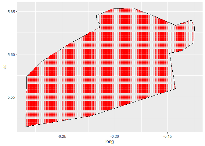
nrow(points_in_polygon)
## [1] 13601
Now there are only 13,601 point left. The next part of code will take some time to run as it needs to calculate the traveling distance/time from 13,601 locations to 315 bars (4,284,315 routes in total), and pick the shortest travel time. There are definitely ways to optimize this code (for example, I could decide to only calculate the route to the 10 Great-circle distance nearest bars and calculate travel times form them). But I only intend to run this code once, and computers are patient workers. I do split the points in some different sections, to limit the complexity on the OSRM server a bit.
# Split data in to chunks of 500
points_in_polygon$section <- rep(1:ceiling(nrow(points_in_polygon)/500), each=500)[1:nrow(points_in_polygon)]


# create an empty list
list_points <- list()

# iterate of the different 500 point chunks
for(i in unique(points_in_polygon$section)){

  # select current chunk
  data_points <- points_in_polygon %>%
  filter(section == i) %>%
  select(-section)

  # this is the OSRM function that calculates the travel time
  travel_time_story <- osrmTable(src = data_points,
                                 dst = bar_locations_lat_long,
                                 measure = "duration")

  # for every point the function calculates the travel time to every bar
  # I only need to save the walking duration to the nearest bar
  list_points[[i]] <- bind_cols(travel_time_story$sources,
                                 mintime = apply(travel_time_story$durations, 1, min)) %>%
    as_tibble()

}

# for points with more than 1 hour walking distance, I cap them at 1 hour (for plotting purposes)
# I also bind the travel duration back on to the original grid
points_in_polygon_with_travel_times <- data.table::rbindlist(list_points) %>%
  mutate(mintime_capped = ifelse(mintime > 60, 60, mintime)) %>%
  bind_cols(points_in_polygon %>%
              select(lon, lat) %>%
              rename(lon.org = lon,
                     lat.org = lat))
If I plot this, this is how it looks, It starts resembling what I am looking for.
ggplot() +
  geom_polygon(data = accra_boundries_poly,
               aes(x=long, y=lat, group = group),
               fill = NA, col = "black") +
  geom_point(data = points_in_polygon_with_travel_times,
             aes(x = lon.org, y = lat.org, col = mintime_capped), size = .1) +
  viridis::scale_color_viridis(option = "magma", direction = -1) +
  geom_point(data = bar_locations_lat_long,
             aes(x = lon, y = lat), col = "blue", size = 3, shape = 10)
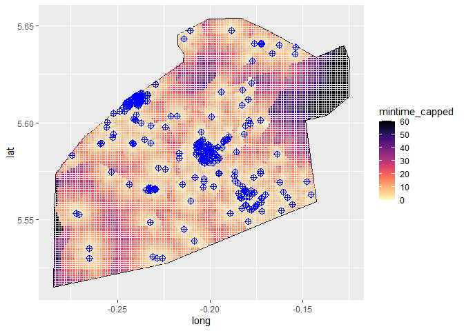
The mean and median walking time (in minutes) from any given point in Accra, Ghana to the nearest bar from that point can be calculated as:
mean(points_in_polygon_with_travel_times$mintime)
## [1] 17.13582
median(points_in_polygon_with_travel_times$mintime)
## [1] 12.8
Not bad!
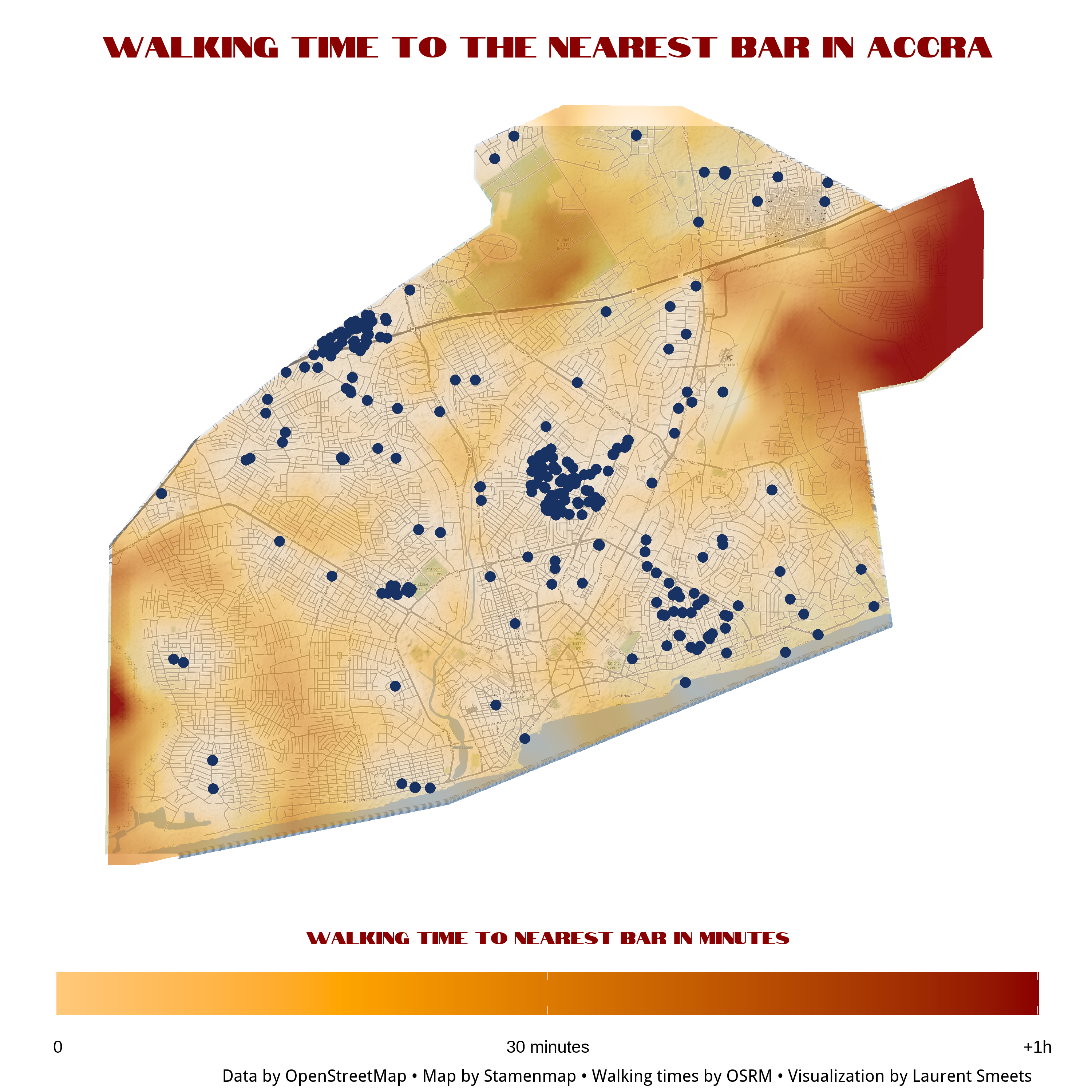
Beautify the Plot
Now I just need to make a raster file out of these points, interpolate between points, project it over a real map of Accra, and make the plot a bit more beautiful.
# set a resolution
gridRes  <- 5

# transform data to SpatialPointsDataFrame  with longitude/latitude projection
data_sp <- points_in_polygon_with_travel_times
coordinates(data_sp) <- ~lon.org+lat.org
proj4string(data_sp) <- crs("+init=epsg:4326")
coords <- c("lon", "lat")

data_sf <- st_as_sf(data_sp, coords = coords, crs = proj4string(data_sp))

# Reset it to the projection of Ghana
data_sp_mp <- spTransform(data_sp, CRSobj = CRS_string)


# Here I set the bounding box I want to use (plus a bit of a margin)
# I also create a new grid that is used for the interpolation

boxx = data_sp_mp@bbox
deltaX = as.integer((boxx[1,2] - boxx[1,1]) + 1.5)
deltaY = as.integer((boxx[2,2] - boxx[2,1]) + 1.5)
gridSizeX = deltaX / gridRes
gridSizeY = deltaY / gridRes
grd = GridTopology(boxx[,1], c(gridRes,gridRes), c(gridSizeX,gridSizeY))
pts = SpatialPoints(coordinates(grd))


# Reset it to the projection of Ghana
proj4string(pts) <- crs(CRS_string)

# create an empty raster
r.raster <- raster::raster()
# set the extent of the raster to the data points I used
extent(r.raster) <- extent(pts)
# set the resolution (cell size)
res(r.raster) <- gridRes
# set the correct crs
crs(r.raster) <- crs(CRS_string) #

# Interpolate the grid cells Nearest neighbour function (k = 20) using the gstat package
gs <- gstat(formula = mintime_capped~1,
            locations = data_sp_mp,
            nmax = 20,
            set = list(idp = 0))

# This might take a while to run
raster_object <- interpolate(r.raster, gs)

# ad both object to a list
minraster <- list(data_sf, raster_object)
names(minraster) <- c("data", "raster_object")

accra_boundries_t <- spTransform(accra_boundries, CRSobj = CRS_string)
minraster_shaped <- mask(minraster$raster_object, accra_boundries_t)
To plot this in ggplot2 I need to make a polygon object out of the raster object.
# you could use this code to speed up the plotting.

 minraster_shaped_aggr <- aggregate(minraster_shaped, fact = 4)
# again, this function might take a while to run
# if it takes to long, set a higher aggregation factor
# or a higher gridres
# or less points


minraster_shaped_rtp <- rasterToPolygons(minraster_shaped_aggr)

# go back to standard long/lat projection for plotting purposes
minraster_shaped_rtp <- spTransform(minraster_shaped_rtp,
                                    CRS("+proj=longlat +datum=WGS84 +no_defs +ellps=WGS84 +towgs84=0,0,0"))

# Now I fortify this data to plot it
minraster_shaped_rtp@data$id <- 1:nrow(minraster_shaped_rtp@data)
minraster_shaped_fort <- fortify(minraster_shaped_rtp,
                                 data = minraster_shaped_rtp@data)
minraster_shaped_fort <- merge(minraster_shaped_fort,
                               minraster_shaped_rtp@data,
                               by.x = 'id',
                               by.y = 'id')
I would like to have some real map as a background, so I download it from Stamenmap and use a function I found here to crop out a polygon and plot the result.
# download background map tiles
# for this level of zoom, you might have to run this command a few times
Accra_city_map <- get_stamenmap(bbox = accra_boundries@bbox, maptype = "terrain", zoom = 15, crop = F)

# load the function to make a raster file out of the tiles
ggmap_rast <- function(map){
  map_bbox <- attr(map, 'bb')
  .extent <- extent(as.numeric(map_bbox[c(2,4,1,3)]))
  my_map <- raster(.extent, nrow= nrow(map), ncol = ncol(map))
  rgb_cols <- setNames(as.data.frame(t(col2rgb(map))), c('red','green','blue'))
  red <- my_map
  values(red) <- rgb_cols[['red']]
  green <- my_map
  values(green) <- rgb_cols[['green']]
  blue <- my_map
  values(blue) <- rgb_cols[['blue']]
  stack(red,green,blue)
}

# make a raster file out of the maps
Accra_city_map_rast <- ggmap_rast(Accra_city_map)

# crop the raster file
Accra_city_map_crop_masked <- mask(Accra_city_map_rast, accra_boundries, inverse=F)

# create a geospatial dataframe out of the raster file
Accra_city_map_crop_masked_df <- data.frame(rasterToPoints(Accra_city_map_crop_masked))

sysfonts::font_add_google("Notable", "Notable") # this is the font I will be using

#These are needed to render the fonts
showtext_auto()
x11()

# create the map in ggplot
static_map  <- ggplot() +
  geom_point(data = Accra_city_map_crop_masked_df,
             aes(x = x,
                 y = y,
                 col = rgb(layer.1/255,
                           layer.2/255,
                           layer.3/255))) +
  scale_color_identity() +
  geom_polygon(data = minraster_shaped_fort,
               aes(x = long,
                   y = lat,
                   group = group,
                   fill = var1.pred,
                   alpha = var1.pred),
               size = 0) +
  coord_map() +
  scale_fill_gradient2(high = "darkred",
                       mid = "orange",
                       low = "white",
                       midpoint = mean(points_in_polygon_with_travel_times$mintime),
                       name = "Walking time to nearest bar in minutes",
                       limits = c(0, 60),
                       breaks = c(0, 30,  60),
                       labels = c("0","30 minutes",  "+1h"),
                       guide = guide_colorbar(
                         direction = "horizontal",
                         barheight = unit(10, units = "mm"),
                         barwidth = unit(9, units = "inch"),
                         draw.ulim = T,
                         title.position = 'top',
                         title.hjust = 0.5,
                         label.hjust = 0.5,
                         legend.location = "bottom"))+
  scale_alpha_continuous(guide = "none",
                         range = c(0.2,.9)) +
  geom_point(data = bar_locations_lat_long,
             aes(x = lon,
                 y = lat),
             col = "#193264FF",
             size = 3,
             shape = 16) +
  ggthemes::theme_map() +
  theme(legend.position = "bottom",
        plot.title = element_markdown(family = "Notable",
                                      size = 60,
                                      face = "bold",
                                      hjust = 0.5,
                                      color = "darkred",
                                      margin = margin(t = 20, b = 2)),
        legend.title = element_markdown(family = "Notable", color = "darkred", size = 35),
        legend.text = element_text(size = 35),
        plot.caption = element_text(size = 35)) +
  labs(title = "Walking Time to the Nearest Bar in Accra",
       caption = "Data by OpenStreetMap • Map by Stamenmap • Walking times by OSRM • Visualization by Laurent Smeets",
       x = NULL,
       y = NULL)

# Do not save this is a .PDF, the raster file as a polygon, is HUGE in a vector file format
ggsave("static_map.png", static_map, width = 10, height = 10, dpi = 300)
This is how the plot looks now. The blue dots indicate the location of the different bars.
Ghana Data Stuff
This website is my hobby project to showcase some of the project I am working one, when I am not working on the official statistics at the Ghana Statistical Service.