Finding the Greenest Neigbourhood in Accra Using Open-source Satellite Sentinel-2 NDVI Data

Introduction
Trees are healthy and people in neighbourhoods live longer. I am absolutely not a health expert, but still, I would like to live in a green neighbourhood. This blog will show you how to calculate the average ‘greenness’ of a neighbourhood using open-sources (or at least free) satellite imagery.
At any given time, multiple satellites are scanning our planet using different instruments. A lot of the data these satellites relay back to earth are openly accessible via USGS (United States Geological Survey) or ESA (European Space Agency). In addition to ‘simply’ taking pictures, satellites register different wavelengths of spectral images. The Landsat-8 mission by NASA and USGS scans our planet every 16 days and takes spectral images at a spatial resolution of 30 meters (so every pixel is 30m by 30m). The data can easily be accessed and viewed here. The Sentinel-2 mission by the ESA, completes scanning the earth every 10 days and creates spectral images at a spatial resolution of 10 meters (so every pixel is 10m by 10m). There are quite some technical differences between the kind of images these two missions create and the instruments they use to do so. If this is a wormhole you want to dive in, just Google “Sentinel vs. Landsat”, but a good place to start is here or here. For now it is just important to know is that both can be used to calculate the so-called Normalized Difference Vegetation Index or NDVI. The NDVI is the main method researchers use to estimate how ‘green’ or forested a certain place is. This index makes use of the fact that, compared to most other surfaces, ‘the pigment in plant leaves, chlorophyll, strongly absorbs visible light (from 0.4 to 0.7 µm) for use in photosynthesis, while cell structure of the leaves, on the other hand, strongly reflects near-infrared light (from 0.7 to 1.1 µm). The more leaves a plant has, the more these wavelengths of light are affected, respectively.' Source and a longer explanation can be found here. So, to calculate a measure of the greenness of a pixel in a satellite image, we can make use of the NDVI formula:
$$ NDVI= \frac{\text{near infrared light - red light}}{\text{near infrared light + red light}} $$
This means that for every pixel in a satellite image I get a value NDVI value between -1 and 1. Roughly summarized, negative values of the NDVI indicate water, low value around 0 indicate urban or dry areas, values from 0.2 to .3 shrubs and meadows, and large values (from 0.6 to 0.8) indicate temperate and tropical forests.
The nice things about both the Landsat data (by default a .tif file) and the Sentinel data (by default a .jp2 file) are that they can be easily imported into R as a raster file. A raster file is basically a very big matrix of rows and columns and values in the cells. This makes manipulations of the data very fast in R and easy to understand. I have listed some tutorials and other readings at the bottom of this page if you want to know more about raster files and how to work with them (in R).
In this post, I will make use of the new getSpatialData
package to download the data I want. This package makes it easy to download both Sentinel and Landsat data directly from R and create make sure you get the right tiles (pictures).
Packages
library(getSpatialData)
library(raster)
library(sf)
library(sp)
library(tidyverse)
library(ggrepel)
library(scales)
library(ggmap)
library(ggridges)
library(showtext)
library(ggtext)
library(cartography)
library(png)
library(kableExtra)

# add a font I will be using
font_add_google(name = "Raleway", regular.wt = 300)
Define Neighbourhoods
As I said, I want to calculate the average greenness of the different neighbourhoods in Accra, Ghana. Before I get into downloading satellite data, I need to define the different neighbourhoods of Accra. I found this interesting paper by Engstrom, Ofiesh, Rain, Jewell and Weeks and used the same shapefile as the authors did (based on the 2010 Ghana census).
# load the shape file both as sf and  SpatialPolygonsDataFrame
Accra_Neigborhoods <- st_read("AccraFMVs2010.shp", quiet = TRUE)
Accra_Neigborhoods_df <- rgdal::readOGR("AccraFMVs2010.shp", layer= "AccraFMVs2010", verbose=FALSE)
ggplot(Accra_Neigborhoods) +
  geom_sf(aes(fill = Popul_2010), colour="grey") +
  coord_sf() +
  theme_minimal() +
  ggrepel::geom_label_repel(
    aes(label = FMV_Name, geometry = geometry),
    stat = "sf_coordinates",
    alpha = .8,
    min.segment.length = 0
  )+
  scale_fill_viridis_c(labels = comma) +
  labs(x = NULL,
       y = NULL,
       fill = "Population",
       title = "Names of Neighbourhoods in Accra, Ghana",
       subtitle = "colour shaded by population in 2010")
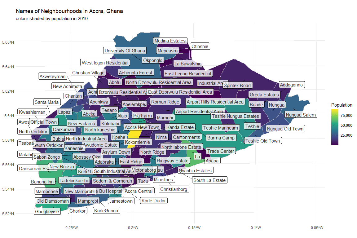
This somewhat chaotic plot shows the 100 different neighbourhoods of Accra.
nrow(Accra_Neigborhoods) # number of different shapes (neighbourhoods)
## [1] 100
To download the right satellite data I need to combine the different shapefiles into one shapefile of Accra.
Accra <- Accra_Neigborhoods %>%
  summarise(area = sum(Shape_Area))
Accra
## Simple feature collection with 1 feature and 1 field
## geometry type:  POLYGON
## dimension:      XY
## bbox:           xmin: 800942.9 ymin: 610718.6 xmax: 826279 ymax: 627180.8
## projected CRS:  WGS 84 / UTM zone 30N
##        area                       geometry
## 1 225126529 POLYGON ((809304.8 612826.2...
Now I have the right shapefile to start the process of downloading the right satellite image. To download Landsat-8 data files from the right API, you need a USGS EROS account (register at: https://ers.cr.usgs.gov/register/) and to download Sentinel data you need a Copernicus Scihub Open Access account (register at: https://scihub.copernicus.eu/). Both of these are free and take like 5 minutes to create.
login_USGS(username = "My_USGS_username", password = "My_USGS_Password")
login_CopHub(username = "My_CopHub_username", password = "My_CopHub_Password")
## Login successfull. USGS ERS credentials have been saved for the current session.
## Login successfull. ESA Copernicus credentials have been saved for the current session.
Now I am ready to start querying some data. The getSpatialData package, makes use of a workflow that is described ob the package’s
Github page. First I define the area of interest (aoi), using the set_aoi() function. In my case that are the boundaries of Accra. After that, I can define which platform I would like to download. If you want to see all the platforms and products that are available, you can use get_products() command. I also specify that I am only interested in images that were taken between October 2019 and January 2020. That, at least last year were the months between the Rain Season and the
harmattan. This seen the optimal months to determine how green Accra was to me.
set_aoi(st_geometry(Accra))
records_Accra_Oct_Dec_2019 <- get_records(time_range = c("2019-10-01", "2020-01-01"),
                                          platform = c("Sentinel-2", "LANDSAT_8_C1"))
In total there are 244 images I could now pick from. I will select a single Sentinel image. For this specific purpose the difference between 30m and 10m spatial resolution is quite noticeable, which is why I prefer the Sentinel Image for now. All the following procedures could easily be done with Landsat data as well.
Download Sentinel Images
It is often quite cloudy in Accra, so I can filter out all the images with a high cloud coverage. I also can plot the outline of the satellite images to check whether they completely contain Accra. It is possible to combine different overlapping images into one, but in this case, it is easier to just find an image that completely covers Accra.
Sentinel_file <- records_Accra_Oct_Dec_2019 %>%
  filter(product_group == "Sentinel") %>% # filter only sentinel images
  filter(as.numeric(cloudcov) < 2) # filter only images with less than 2% cloud coverage
for(i in 1:nrow(Sentinel_file)){
p <- plot_records(Sentinel_file[i,]) +
  theme(legend.position = "bottom")

print(p)
}
## Composing preview plot...
## Composing preview plot...
## Composing preview plot...
## Composing preview plot...
## Composing preview plot...
## Composing preview plot...
## Composing preview plot...
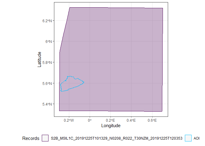
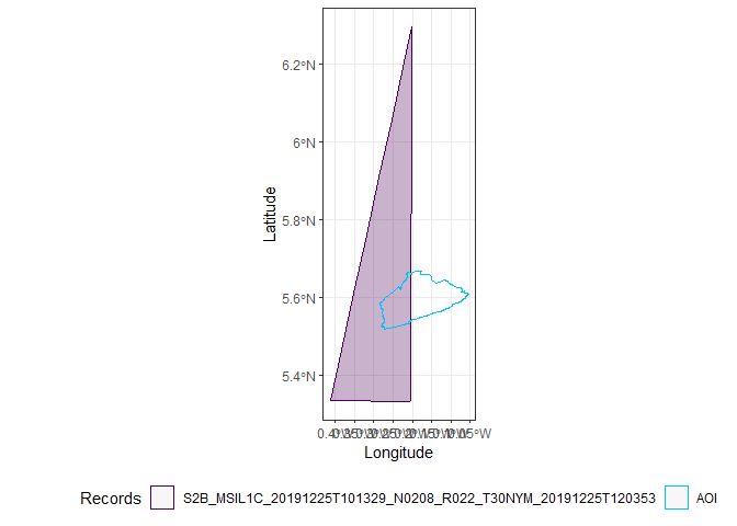
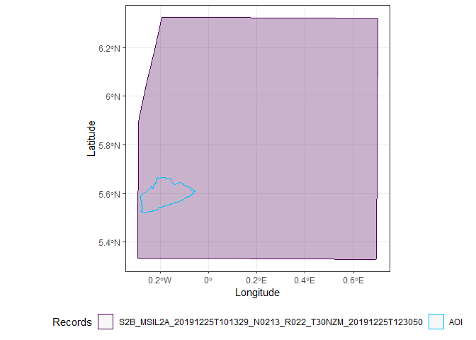

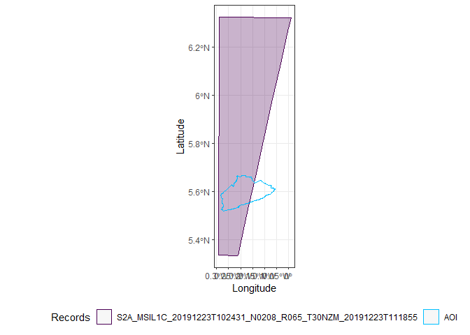
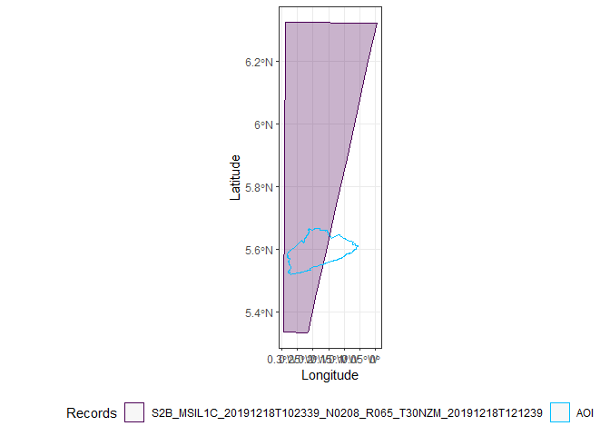
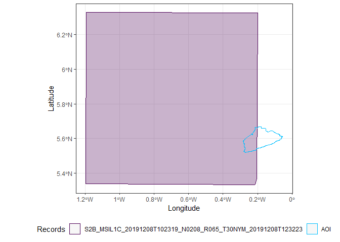
Only two images completely cover Accra, the first and the third.
Sentinel_file <- Sentinel_file %>%
  slice(1,3) # select the 1st and 3rd file
Sentinel_file
## Simple feature collection with 2 features and 35 fields
## geometry type:  MULTIPOLYGON
## dimension:      XY
## bbox:           xmin: -0.2935181 ymin: 5.328635 xmax: 0.7024217 ymax: 6.325381
## geographic CRS: WGS 84
##   product_group    product
## 1      Sentinel Sentinel-2
## 2      Sentinel Sentinel-2
##                                                      record_id
## 1 S2B_MSIL1C_20191225T101329_N0208_R022_T30NZM_20191225T120353
## 2 S2B_MSIL2A_20191225T101329_N0213_R022_T30NZM_20191225T123050
##                              entity_id
## 1 78bf521b-c764-4b46-a5cc-053f4c7ac4a2
## 2 d45e3eda-1023-4188-b9d8-125866613408
##                                                                                           summary
## 1 Date: 2019-12-25T10:13:29.024Z, Instrument: MSI, Mode: , Satellite: Sentinel-2, Size: 675.30 MB
## 2 Date: 2019-12-25T10:13:29.024Z, Instrument: MSI, Mode: , Satellite: Sentinel-2, Size: 955.02 MB
##   date_acquisition               start_time                stop_time
## 1       2019-12-25 2019-12-25T10:13:29.024Z 2019-12-25T10:13:29.024Z
## 2       2019-12-25 2019-12-25T10:13:29.024Z 2019-12-25T10:13:29.024Z
##             date_ingestion date_modified tile_id tile_number_horizontal
## 1 2019-12-25T16:57:07.491Z          <NA>   30NZM                     NA
## 2 2019-12-25T16:03:56.234Z          <NA>   30NZM                     NA
##   tile_number_vertical
## 1                   NA
## 2                   NA
##                                                                                                             md5_url
## 1 https://scihub.copernicus.eu/dhus/odata/v1/Products('78bf521b-c764-4b46-a5cc-053f4c7ac4a2')/Checksum/Value/$value
## 2 https://scihub.copernicus.eu/dhus/odata/v1/Products('d45e3eda-1023-4188-b9d8-125866613408')/Checksum/Value/$value
##                                                                                                                preview_url
## 1 https://scihub.copernicus.eu/dhus/odata/v1/Products('78bf521b-c764-4b46-a5cc-053f4c7ac4a2')/Products('Quicklook')/$value
## 2 https://scihub.copernicus.eu/dhus/odata/v1/Products('d45e3eda-1023-4188-b9d8-125866613408')/Products('Quicklook')/$value
##   meta_url meta_url_fgdc orbit_number orbit_direction relativeorbit_number
## 1     <NA>          <NA>        14634      DESCENDING                   22
## 2     <NA>          <NA>        14634      DESCENDING                   22
##   product_type   platform platform_id platform_serial                    sensor
## 1      S2MSI1C Sentinel-2   2017-013A     Sentinel-2B Multi-Spectral Instrument
## 2      S2MSI2A Sentinel-2   2017-013A     Sentinel-2B Multi-Spectral Instrument
##   sensor_id sensor_mode      size is_gnss cloudcov_land cloudcov    level
## 1       MSI    INS-NOBS 675.30 MB   FALSE            NA  0.29890 Level-1C
## 2       MSI        <NA> 955.02 MB   FALSE            NA  1.17594 Level-2A
##   processingbaseline cloudcov.1 ImageQuality                      footprint
## 1              02.08       <NA>           NA MULTIPOLYGON (((0.6959279 5...
## 2              02.13       <NA>           NA MULTIPOLYGON (((0.6959279 5...
Both images were taken on 2019-12-25, one using level 1C and one using level 2A. There is really not that much difference between the two, at least for my purposes, so, for now, I will just use the one using level 2A.
Sentinel_file <- Sentinel_file %>%
  filter(level == "Level-2A") # only keep this record.
Now I go proceed with downloading the actual data. As you can see, this is a big file (955MB), which is why it is important that you make sure you want to download the file.
set_archive("./data/")
Sentinel_file  <- order_data(Sentinel_file)
Sentinel_file <- get_data(Sentinel_file)
All placed orders are now available for download.
Receiving MD5 checksums...
Assembling dataset URLs...
[Dataset 1/1 | File 1/1] Downloading dataset 'S2B_MSIL2A_20191225T101329_N0213_R022_T30NZM_20191225T123050 (Level-2A)' to './data/_datasets/Sentinel-2//S2B_MSIL2A_20191225T101329_N0213_R022_T30NZM_20191225T123050.zip'...
  |==                                                                                                                                    |   2%
Unzip Sentinel Images
These are all the files that are now in the data folder
list.files("./data/", recursive = T)
## [1] "_datasets/Sentinel-2/S2B_MSIL2A_20191225T101329_N0213_R022_T30NZM_20191225T123050.zip"
Then I unzip the files that were downloaded.
unzip("./data/_datasets/Sentinel-2/S2B_MSIL2A_20191225T101329_N0213_R022_T30NZM_20191225T123050.zip", exdir = getwd())
These are the different files I downloaded with this request (131 in total).
list.files("./S2B_MSIL2A_20191225T101329_N0213_R022_T30NZM_20191225T123050.SAFE", recursive = T) %>%
  kable() %>%
  kable_styling(c("striped", "hover", "condensed")) %>%
  scroll_box(width = "100%", height = "300px")
| x |
|---|
| DATASTRIP/DS_SGS__20191225T123050_S20191225T102600/MTD_DS.xml |
| DATASTRIP/DS_SGS__20191225T123050_S20191225T102600/QI_DATA/FORMAT_CORRECTNESS.xml |
| DATASTRIP/DS_SGS__20191225T123050_S20191225T102600/QI_DATA/GENERAL_QUALITY.xml |
| DATASTRIP/DS_SGS__20191225T123050_S20191225T102600/QI_DATA/GEOMETRIC_QUALITY.xml |
| DATASTRIP/DS_SGS__20191225T123050_S20191225T102600/QI_DATA/RADIOMETRIC_QUALITY.xml |
| DATASTRIP/DS_SGS__20191225T123050_S20191225T102600/QI_DATA/SENSOR_QUALITY.xml |
| GRANULE/L2A_T30NZM_A014634_20191225T102600/AUX_DATA/AUX_ECMWFT |
| GRANULE/L2A_T30NZM_A014634_20191225T102600/IMG_DATA/R10m/T30NZM_20191225T101329_AOT_10m.jp2 |
| GRANULE/L2A_T30NZM_A014634_20191225T102600/IMG_DATA/R10m/T30NZM_20191225T101329_B02_10m.jp2 |
| GRANULE/L2A_T30NZM_A014634_20191225T102600/IMG_DATA/R10m/T30NZM_20191225T101329_B03_10m.jp2 |
| GRANULE/L2A_T30NZM_A014634_20191225T102600/IMG_DATA/R10m/T30NZM_20191225T101329_B04_10m.jp2 |
| GRANULE/L2A_T30NZM_A014634_20191225T102600/IMG_DATA/R10m/T30NZM_20191225T101329_B08_10m.jp2 |
| GRANULE/L2A_T30NZM_A014634_20191225T102600/IMG_DATA/R10m/T30NZM_20191225T101329_TCI_10m.jp2 |
| GRANULE/L2A_T30NZM_A014634_20191225T102600/IMG_DATA/R10m/T30NZM_20191225T101329_WVP_10m.jp2 |
| GRANULE/L2A_T30NZM_A014634_20191225T102600/IMG_DATA/R20m/T30NZM_20191225T101329_AOT_20m.jp2 |
| GRANULE/L2A_T30NZM_A014634_20191225T102600/IMG_DATA/R20m/T30NZM_20191225T101329_B02_20m.jp2 |
| GRANULE/L2A_T30NZM_A014634_20191225T102600/IMG_DATA/R20m/T30NZM_20191225T101329_B03_20m.jp2 |
| GRANULE/L2A_T30NZM_A014634_20191225T102600/IMG_DATA/R20m/T30NZM_20191225T101329_B04_20m.jp2 |
| GRANULE/L2A_T30NZM_A014634_20191225T102600/IMG_DATA/R20m/T30NZM_20191225T101329_B05_20m.jp2 |
| GRANULE/L2A_T30NZM_A014634_20191225T102600/IMG_DATA/R20m/T30NZM_20191225T101329_B06_20m.jp2 |
| GRANULE/L2A_T30NZM_A014634_20191225T102600/IMG_DATA/R20m/T30NZM_20191225T101329_B07_20m.jp2 |
| GRANULE/L2A_T30NZM_A014634_20191225T102600/IMG_DATA/R20m/T30NZM_20191225T101329_B11_20m.jp2 |
| GRANULE/L2A_T30NZM_A014634_20191225T102600/IMG_DATA/R20m/T30NZM_20191225T101329_B12_20m.jp2 |
| GRANULE/L2A_T30NZM_A014634_20191225T102600/IMG_DATA/R20m/T30NZM_20191225T101329_B8A_20m.jp2 |
| GRANULE/L2A_T30NZM_A014634_20191225T102600/IMG_DATA/R20m/T30NZM_20191225T101329_SCL_20m.jp2 |
| GRANULE/L2A_T30NZM_A014634_20191225T102600/IMG_DATA/R20m/T30NZM_20191225T101329_TCI_20m.jp2 |
| GRANULE/L2A_T30NZM_A014634_20191225T102600/IMG_DATA/R20m/T30NZM_20191225T101329_WVP_20m.jp2 |
| GRANULE/L2A_T30NZM_A014634_20191225T102600/IMG_DATA/R60m/T30NZM_20191225T101329_AOT_60m.jp2 |
| GRANULE/L2A_T30NZM_A014634_20191225T102600/IMG_DATA/R60m/T30NZM_20191225T101329_B01_60m.jp2 |
| GRANULE/L2A_T30NZM_A014634_20191225T102600/IMG_DATA/R60m/T30NZM_20191225T101329_B02_60m.jp2 |
| GRANULE/L2A_T30NZM_A014634_20191225T102600/IMG_DATA/R60m/T30NZM_20191225T101329_B03_60m.jp2 |
| GRANULE/L2A_T30NZM_A014634_20191225T102600/IMG_DATA/R60m/T30NZM_20191225T101329_B04_60m.jp2 |
| GRANULE/L2A_T30NZM_A014634_20191225T102600/IMG_DATA/R60m/T30NZM_20191225T101329_B05_60m.jp2 |
| GRANULE/L2A_T30NZM_A014634_20191225T102600/IMG_DATA/R60m/T30NZM_20191225T101329_B06_60m.jp2 |
| GRANULE/L2A_T30NZM_A014634_20191225T102600/IMG_DATA/R60m/T30NZM_20191225T101329_B07_60m.jp2 |
| GRANULE/L2A_T30NZM_A014634_20191225T102600/IMG_DATA/R60m/T30NZM_20191225T101329_B09_60m.jp2 |
| GRANULE/L2A_T30NZM_A014634_20191225T102600/IMG_DATA/R60m/T30NZM_20191225T101329_B11_60m.jp2 |
| GRANULE/L2A_T30NZM_A014634_20191225T102600/IMG_DATA/R60m/T30NZM_20191225T101329_B12_60m.jp2 |
| GRANULE/L2A_T30NZM_A014634_20191225T102600/IMG_DATA/R60m/T30NZM_20191225T101329_B8A_60m.jp2 |
| GRANULE/L2A_T30NZM_A014634_20191225T102600/IMG_DATA/R60m/T30NZM_20191225T101329_SCL_60m.jp2 |
| GRANULE/L2A_T30NZM_A014634_20191225T102600/IMG_DATA/R60m/T30NZM_20191225T101329_TCI_60m.jp2 |
| GRANULE/L2A_T30NZM_A014634_20191225T102600/IMG_DATA/R60m/T30NZM_20191225T101329_WVP_60m.jp2 |
| GRANULE/L2A_T30NZM_A014634_20191225T102600/MTD_TL.xml |
| GRANULE/L2A_T30NZM_A014634_20191225T102600/QI_DATA/FORMAT_CORRECTNESS.xml |
| GRANULE/L2A_T30NZM_A014634_20191225T102600/QI_DATA/GENERAL_QUALITY.xml |
| GRANULE/L2A_T30NZM_A014634_20191225T102600/QI_DATA/GEOMETRIC_QUALITY.xml |
| GRANULE/L2A_T30NZM_A014634_20191225T102600/QI_DATA/MSK_CLDPRB_20m.jp2 |
| GRANULE/L2A_T30NZM_A014634_20191225T102600/QI_DATA/MSK_CLDPRB_60m.jp2 |
| GRANULE/L2A_T30NZM_A014634_20191225T102600/QI_DATA/MSK_CLOUDS_B00.gml |
| GRANULE/L2A_T30NZM_A014634_20191225T102600/QI_DATA/MSK_DEFECT_B01.gml |
| GRANULE/L2A_T30NZM_A014634_20191225T102600/QI_DATA/MSK_DEFECT_B02.gml |
| GRANULE/L2A_T30NZM_A014634_20191225T102600/QI_DATA/MSK_DEFECT_B03.gml |
| GRANULE/L2A_T30NZM_A014634_20191225T102600/QI_DATA/MSK_DEFECT_B04.gml |
| GRANULE/L2A_T30NZM_A014634_20191225T102600/QI_DATA/MSK_DEFECT_B05.gml |
| GRANULE/L2A_T30NZM_A014634_20191225T102600/QI_DATA/MSK_DEFECT_B06.gml |
| GRANULE/L2A_T30NZM_A014634_20191225T102600/QI_DATA/MSK_DEFECT_B07.gml |
| GRANULE/L2A_T30NZM_A014634_20191225T102600/QI_DATA/MSK_DEFECT_B08.gml |
| GRANULE/L2A_T30NZM_A014634_20191225T102600/QI_DATA/MSK_DEFECT_B09.gml |
| GRANULE/L2A_T30NZM_A014634_20191225T102600/QI_DATA/MSK_DEFECT_B10.gml |
| GRANULE/L2A_T30NZM_A014634_20191225T102600/QI_DATA/MSK_DEFECT_B11.gml |
| GRANULE/L2A_T30NZM_A014634_20191225T102600/QI_DATA/MSK_DEFECT_B12.gml |
| GRANULE/L2A_T30NZM_A014634_20191225T102600/QI_DATA/MSK_DEFECT_B8A.gml |
| GRANULE/L2A_T30NZM_A014634_20191225T102600/QI_DATA/MSK_DETFOO_B01.gml |
| GRANULE/L2A_T30NZM_A014634_20191225T102600/QI_DATA/MSK_DETFOO_B02.gml |
| GRANULE/L2A_T30NZM_A014634_20191225T102600/QI_DATA/MSK_DETFOO_B03.gml |
| GRANULE/L2A_T30NZM_A014634_20191225T102600/QI_DATA/MSK_DETFOO_B04.gml |
| GRANULE/L2A_T30NZM_A014634_20191225T102600/QI_DATA/MSK_DETFOO_B05.gml |
| GRANULE/L2A_T30NZM_A014634_20191225T102600/QI_DATA/MSK_DETFOO_B06.gml |
| GRANULE/L2A_T30NZM_A014634_20191225T102600/QI_DATA/MSK_DETFOO_B07.gml |
| GRANULE/L2A_T30NZM_A014634_20191225T102600/QI_DATA/MSK_DETFOO_B08.gml |
| GRANULE/L2A_T30NZM_A014634_20191225T102600/QI_DATA/MSK_DETFOO_B09.gml |
| GRANULE/L2A_T30NZM_A014634_20191225T102600/QI_DATA/MSK_DETFOO_B10.gml |
| GRANULE/L2A_T30NZM_A014634_20191225T102600/QI_DATA/MSK_DETFOO_B11.gml |
| GRANULE/L2A_T30NZM_A014634_20191225T102600/QI_DATA/MSK_DETFOO_B12.gml |
| GRANULE/L2A_T30NZM_A014634_20191225T102600/QI_DATA/MSK_DETFOO_B8A.gml |
| GRANULE/L2A_T30NZM_A014634_20191225T102600/QI_DATA/MSK_NODATA_B01.gml |
| GRANULE/L2A_T30NZM_A014634_20191225T102600/QI_DATA/MSK_NODATA_B02.gml |
| GRANULE/L2A_T30NZM_A014634_20191225T102600/QI_DATA/MSK_NODATA_B03.gml |
| GRANULE/L2A_T30NZM_A014634_20191225T102600/QI_DATA/MSK_NODATA_B04.gml |
| GRANULE/L2A_T30NZM_A014634_20191225T102600/QI_DATA/MSK_NODATA_B05.gml |
| GRANULE/L2A_T30NZM_A014634_20191225T102600/QI_DATA/MSK_NODATA_B06.gml |
| GRANULE/L2A_T30NZM_A014634_20191225T102600/QI_DATA/MSK_NODATA_B07.gml |
| GRANULE/L2A_T30NZM_A014634_20191225T102600/QI_DATA/MSK_NODATA_B08.gml |
| GRANULE/L2A_T30NZM_A014634_20191225T102600/QI_DATA/MSK_NODATA_B09.gml |
| GRANULE/L2A_T30NZM_A014634_20191225T102600/QI_DATA/MSK_NODATA_B10.gml |
| GRANULE/L2A_T30NZM_A014634_20191225T102600/QI_DATA/MSK_NODATA_B11.gml |
| GRANULE/L2A_T30NZM_A014634_20191225T102600/QI_DATA/MSK_NODATA_B12.gml |
| GRANULE/L2A_T30NZM_A014634_20191225T102600/QI_DATA/MSK_NODATA_B8A.gml |
| GRANULE/L2A_T30NZM_A014634_20191225T102600/QI_DATA/MSK_SATURA_B01.gml |
| GRANULE/L2A_T30NZM_A014634_20191225T102600/QI_DATA/MSK_SATURA_B02.gml |
| GRANULE/L2A_T30NZM_A014634_20191225T102600/QI_DATA/MSK_SATURA_B03.gml |
| GRANULE/L2A_T30NZM_A014634_20191225T102600/QI_DATA/MSK_SATURA_B04.gml |
| GRANULE/L2A_T30NZM_A014634_20191225T102600/QI_DATA/MSK_SATURA_B05.gml |
| GRANULE/L2A_T30NZM_A014634_20191225T102600/QI_DATA/MSK_SATURA_B06.gml |
| GRANULE/L2A_T30NZM_A014634_20191225T102600/QI_DATA/MSK_SATURA_B07.gml |
| GRANULE/L2A_T30NZM_A014634_20191225T102600/QI_DATA/MSK_SATURA_B08.gml |
| GRANULE/L2A_T30NZM_A014634_20191225T102600/QI_DATA/MSK_SATURA_B09.gml |
| GRANULE/L2A_T30NZM_A014634_20191225T102600/QI_DATA/MSK_SATURA_B10.gml |
| GRANULE/L2A_T30NZM_A014634_20191225T102600/QI_DATA/MSK_SATURA_B11.gml |
| GRANULE/L2A_T30NZM_A014634_20191225T102600/QI_DATA/MSK_SATURA_B12.gml |
| GRANULE/L2A_T30NZM_A014634_20191225T102600/QI_DATA/MSK_SATURA_B8A.gml |
| GRANULE/L2A_T30NZM_A014634_20191225T102600/QI_DATA/MSK_SNWPRB_20m.jp2 |
| GRANULE/L2A_T30NZM_A014634_20191225T102600/QI_DATA/MSK_SNWPRB_60m.jp2 |
| GRANULE/L2A_T30NZM_A014634_20191225T102600/QI_DATA/MSK_TECQUA_B01.gml |
| GRANULE/L2A_T30NZM_A014634_20191225T102600/QI_DATA/MSK_TECQUA_B02.gml |
| GRANULE/L2A_T30NZM_A014634_20191225T102600/QI_DATA/MSK_TECQUA_B03.gml |
| GRANULE/L2A_T30NZM_A014634_20191225T102600/QI_DATA/MSK_TECQUA_B04.gml |
| GRANULE/L2A_T30NZM_A014634_20191225T102600/QI_DATA/MSK_TECQUA_B05.gml |
| GRANULE/L2A_T30NZM_A014634_20191225T102600/QI_DATA/MSK_TECQUA_B06.gml |
| GRANULE/L2A_T30NZM_A014634_20191225T102600/QI_DATA/MSK_TECQUA_B07.gml |
| GRANULE/L2A_T30NZM_A014634_20191225T102600/QI_DATA/MSK_TECQUA_B08.gml |
| GRANULE/L2A_T30NZM_A014634_20191225T102600/QI_DATA/MSK_TECQUA_B09.gml |
| GRANULE/L2A_T30NZM_A014634_20191225T102600/QI_DATA/MSK_TECQUA_B10.gml |
| GRANULE/L2A_T30NZM_A014634_20191225T102600/QI_DATA/MSK_TECQUA_B11.gml |
| GRANULE/L2A_T30NZM_A014634_20191225T102600/QI_DATA/MSK_TECQUA_B12.gml |
| GRANULE/L2A_T30NZM_A014634_20191225T102600/QI_DATA/MSK_TECQUA_B8A.gml |
| GRANULE/L2A_T30NZM_A014634_20191225T102600/QI_DATA/RADIOMETRIC_QUALITY.xml |
| GRANULE/L2A_T30NZM_A014634_20191225T102600/QI_DATA/SENSOR_QUALITY.xml |
| GRANULE/L2A_T30NZM_A014634_20191225T102600/QI_DATA/T30NZM_20191225T101329_PVI.jp2 |
| HTML/banner_1.png |
| HTML/banner_2.png |
| HTML/banner_3.png |
| HTML/star_bg.jpg |
| HTML/UserProduct_index.html |
| HTML/UserProduct_index.xsl |
| INSPIRE.xml |
| manifest.safe |
| MTD_MSIL2A.xml |
| rep_info/S2_PDI_Level-2A_Datastrip_Metadata.xsd |
| rep_info/S2_PDI_Level-2A_Tile_Metadata.xsd |
| rep_info/S2_User_Product_Level-2A_Metadata.xsd |
Calculate NDVI from Sentinel-2 Data
All spectral images are saved as different files. As explained
here, the red band for Sentinel-2 data is band 4 and the near-infrared band is band 8. Now I can load in these two bands, using the readGDAL() and transform them into raster files using the raster() function. Once the files are expressed as raster files, I can calculate the NDVI from them using simple matrix manipulations. The images are saved at a different resolution, but I will use the most ‘precise’ one (10m)
# this is the path to the red band
path_to_red_sentinel <- './S2B_MSIL2A_20191225T101329_N0213_R022_T30NZM_20191225T123050.SAFE/GRANULE/L2A_T30NZM_A014634_20191225T102600/IMG_DATA/R10m/T30NZM_20191225T101329_B04_10m.jp2'

# this is the path to the near infrared band
path_to_nearinfrared_sentinel <- './S2B_MSIL2A_20191225T101329_N0213_R022_T30NZM_20191225T123050.SAFE/GRANULE/L2A_T30NZM_A014634_20191225T102600/IMG_DATA/R10m/T30NZM_20191225T101329_B08_10m.jp2'

# load data
red_sentinel <- rgdal::readGDAL(path_to_red_sentinel)
## ./S2B_MSIL2A_20191225T101329_N0213_R022_T30NZM_20191225T123050.SAFE/GRANULE/L2A_T30NZM_A014634_20191225T102600/IMG_DATA/R10m/T30NZM_20191225T101329_B04_10m.jp2 has GDAL driver JP2OpenJPEG
## and has 10980 rows and 10980 columns
nir_sentinel <- rgdal::readGDAL(path_to_nearinfrared_sentinel)
## ./S2B_MSIL2A_20191225T101329_N0213_R022_T30NZM_20191225T123050.SAFE/GRANULE/L2A_T30NZM_A014634_20191225T102600/IMG_DATA/R10m/T30NZM_20191225T101329_B08_10m.jp2 has GDAL driver JP2OpenJPEG
## and has 10980 rows and 10980 columns
# transform data to raster file
red_raster_sentinel <- raster(red_sentinel)
nir_raster_sentinel <- raster(nir_sentinel)

#calculate NDVI
ndvi_sentinel <- ((nir_raster_sentinel - red_raster_sentinel)/(nir_raster_sentinel + red_raster_sentinel))

# plot NDVI
plot(ndvi_sentinel)
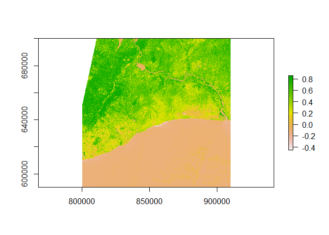
Crop the Data to Neighbourhood Shapefiles
Clearly, I have downloaded a photo that is much bigger than just Accra, so now I subset a small piece of this picture. I would like to have some real map as a background, so I download it from Stamenmap and use a function I found here to crop out a polygon and plot the result.
# set projection WS84 mercator projection
projection_long_lat <- CRS('+proj=longlat +ellps=WGS84 +datum=WGS84 +no_defs')
Accra_Neigborhoods_df2 <- spTransform(Accra_Neigborhoods_df, projection_long_lat)
ndvi_merc <- projectRaster(ndvi_sentinel, crs = projection_long_lat)

# crop and mask square NDVI image to just outline of Accra
ndvi_merc_cropped <- crop(ndvi_merc, Accra_Neigborhoods_df2)
ndvi_merc_cropped <- mask(ndvi_merc_cropped, Accra_Neigborhoods_df2)

# download background for the plot
bounding_box <- Accra_Neigborhoods_df2@bbox
Accra_map_bg <- get_stamenmap(bbox = bounding_box, zoom = 14,  color = "bw", crop = T)

# load the function to make a raster file out of the tiles
ggmap_rast <- function(map){
  map_bbox <- attr(map, 'bb')
  .extent <- extent(as.numeric(map_bbox[c(2,4,1,3)]))
  my_map <- raster(.extent, nrow= nrow(map), ncol = ncol(map))
  rgb_cols <- setNames(as.data.frame(t(col2rgb(map))), c('red','green','blue'))
  red <- my_map
  values(red) <- rgb_cols[['red']]
  green <- my_map
  values(green) <- rgb_cols[['green']]
  blue <- my_map
  values(blue) <- rgb_cols[['blue']]
  stack(red,green,blue)
}

Accra_map_bg_rast <- ggmap_rast(Accra_map_bg)
Accra_map_bg_rast <- mask(Accra_map_bg_rast, Accra_Neigborhoods_df2)
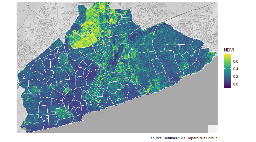
Now I make a plot, with the NDVI raster file, neighbourhood shapefile and map background.
ggmap(Accra_map_bg) +
  geom_raster(data =na.omit(ndvi_merc_cropped),
                aes(x = x, y = y, fill = layer, alpha = ifelse(is.na(layer), 0, .7))) +
  geom_polygon(data = fortify(Accra_Neigborhoods_df2),
                aes(x=long, y=lat, group = group),
                fill = NA, col = "white", size =.6) +
  scale_color_identity() +
  scale_fill_viridis_c(option = "viridis") +
  coord_quickmap()+
  labs(fill = "NDVI",
       caption = "source: Sentinel-2 via Copernicus Scihub")+
  guides(alpha = F) +
  theme_minimal()+
  theme(axis.text = element_blank(),
        axis.title = element_blank())
Statistics
Now I can calculate some NDVI statistics, both for the city as a whole and for individual neighbourhoods.
Accra_stats <- ndvi_merc_cropped %>%
  values() %>% # extract the NDVI values
  na.omit() %>% # omit the missing values (outside of the crop)
  enframe() %>%
    summarise(mean_NDVI = mean(value),
            median_NDVI = median(value),
            NDVI_sd = sd(value),
            NDVI_30_plus = mean(value > .3))

Accra_stats
## # A tibble: 1 x 4
##   mean_NDVI median_NDVI NDVI_sd NDVI_30_plus
##       <dbl>       <dbl>   <dbl>        <dbl>
## 1     0.239       0.187   0.161        0.264
The mean NDVI of Accra (using 10m spatial resolution) is .24, the median .19, the standard deviation .16 and 26.4% of Accra has an NDVI over .3.
Now I can also do this for all the neighbourhoods separately.
list_summary_stats <- list()
list_values <- list()
IDS <- unique(Accra_Neigborhoods_df2$OBJECTID)
for(i in 1:length(IDS)){
 list_summary_stats[[i]] <- ndvi_merc_cropped %>%
    mask(subset(Accra_Neigborhoods_df2, OBJECTID == IDS[i])) %>%
    values() %>%
    na.omit() %>%
    enframe()  %>%
    summarise(mean_NDVI = mean(value),
            median_NDVI = median(value),
            NDVI_sd = sd(value),
            NDVI_30_plus = mean(value > .3),
            Neighbourhood = IDS[i])

 list_values[[i]] <- ndvi_merc_cropped %>%
    mask(subset(Accra_Neigborhoods_df2, OBJECTID == IDS[i])) %>%
    values() %>%
    na.omit() %>%
    enframe()%>%
    mutate(Neighbourhood = IDS[i])
}
# bind values into one dataset and enrich it
df_values <- do.call("rbind", list_values) %>%
  left_join(Accra_Neigborhoods_df2@data %>% dplyr::select(OBJECTID,  FMV_Name),
            by = c("Neighbourhood" = "OBJECTID"))


# bind neighbourhood stats into one dataset and enrich it
df_stats <- do.call("rbind", list_summary_stats) %>%
  left_join(Accra_Neigborhoods_df2@data %>% dplyr::select(OBJECTID,  FMV_Name, HQI_mean, PopDensity),
            by = c("Neighbourhood" = "OBJECTID"))

p_ridges <- df_values %>%
  left_join(df_stats, by = "FMV_Name")%>%
  ggplot(aes(x = value, y = reorder(FMV_Name, mean_NDVI), fill = stat(x)),  alpha = .5) +
  geom_density_ridges_gradient(scale = 3, rel_min_height = 0.01) +
  scale_fill_viridis_c(name = "NDVI", option = "viridis") +
  labs(title = 'NDVI values of 10mx10m tiles\nof different neighbourhoods in Accra',
       caption =   "source: Sentinel-2 via Copernicus Scihub",
       y = NULL,
       x = "NDVI")+
  coord_cartesian(xlim =c(0, 0.8))+
  geom_vline(xintercept = Accra_stats$mean_NDVI) +
  theme_minimal() +
  theme(legend.position = "right",
        plot.title = element_text(family = "Raleway"),
        axis.text = element_text(family = "Raleway"),
        legend.title =element_text(family = "Raleway"),
        legend.text  =element_text(family = "Raleway"),
        plot.caption = element_markdown(family = "Raleway"),
        axis.title = element_markdown(family = "Raleway"))

p_ridges
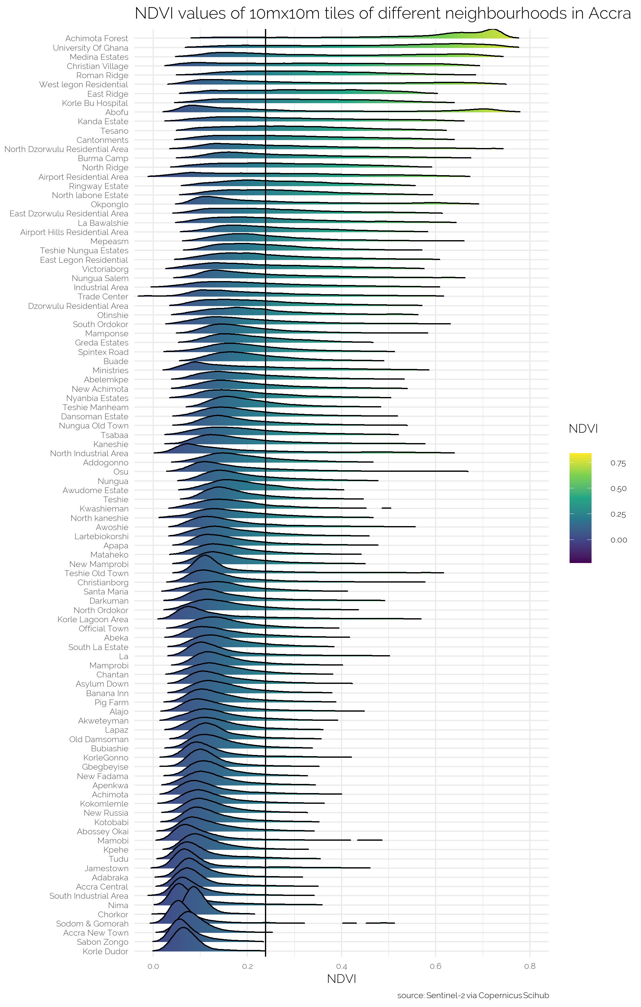
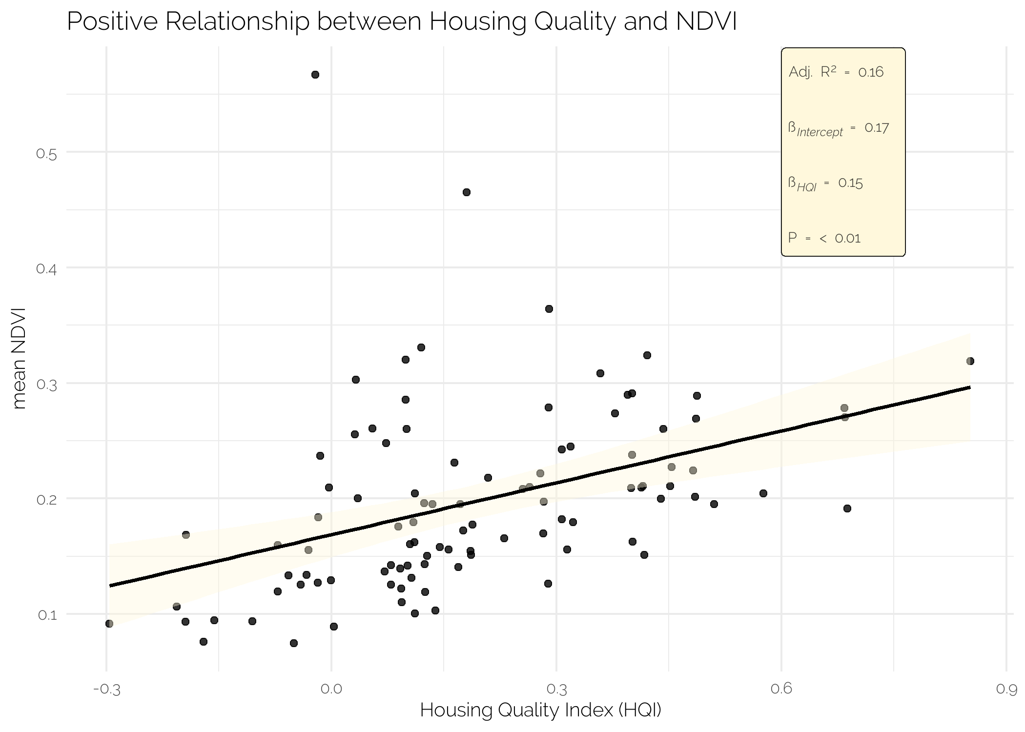
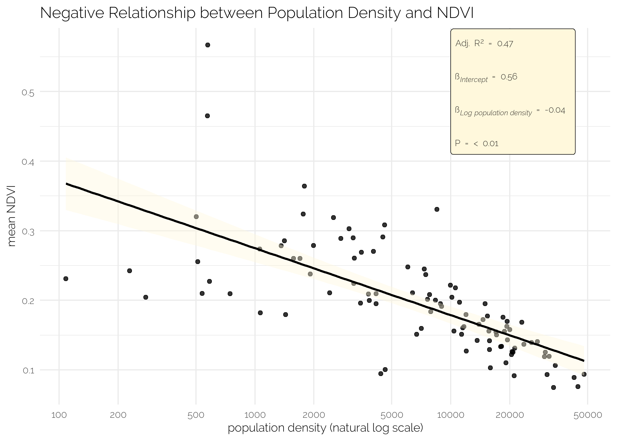
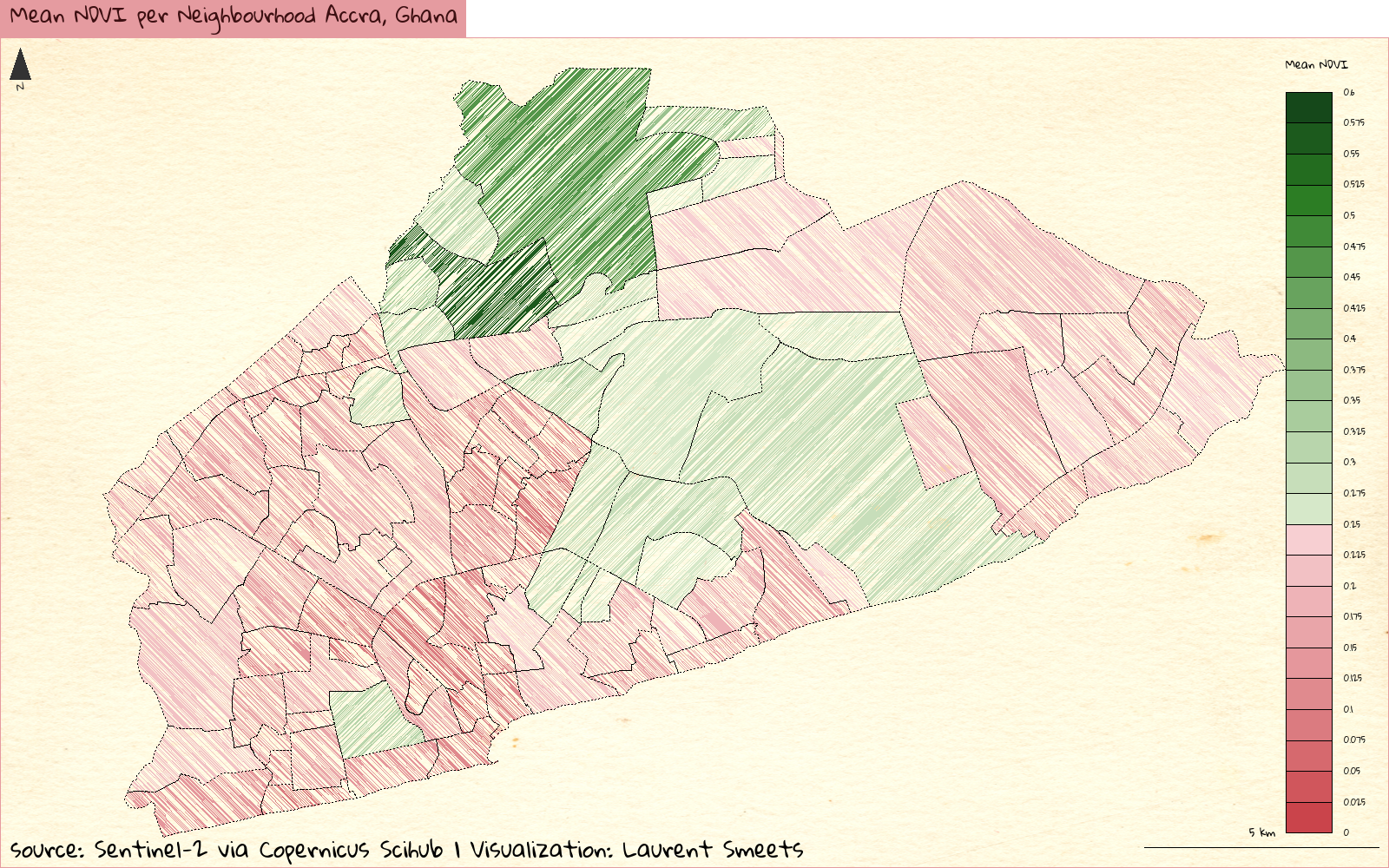
I see that Achimota Forest and the campus of the University of Ghana are the two greenest neighbourhoods and that Sabon Zongo and Korle Dudor are the two least green neighbourhoods on average. Some basic analysis shows that there is a positive relationship between the 2010 mean housing quality of a neigbourhood and the mean NDVI of that neighbourhood and a negative relationship between the (log) population density and mean NDVI. Please note, I do not pretend these easy, short-cut, corn-cutting analyses to be any type of proper analyses or substitution thereof. I did not check for any type of assumption underlying an OLS, nor did I verify any of the data. In all honesty, I do not even know what the housing quality index exactly measures. My educated guess is simply that higher means nicer houses
fit_HQI <- lm(mean_NDVI ~ HQI_mean,  data = df_stats)
fit_logpop <- lm(mean_NDVI ~ log(PopDensity),  data = df_stats)
#These are needed to render the fonts
showtext_auto()
x11()

df_stats %>%
  ggplot(aes(x = HQI_mean, y = mean_NDVI)) +
  geom_point(col = "black", alpha = .8)+
  geom_smooth(method='lm',
              formula  ='y ~ x',,
              se = TRUE,
              col = "black",
              fill = "cornsilk") +
  geom_richtext( x= 0.6,
                 y = 0.5,
                 label = paste("Adj. R<sup>2</sup> = ",round(signif(summary(fit_HQI)$adj.r.squared, 5), 2),"<br>",
                               "β<sub>*Intercept*</sub>  =",round(signif(fit_HQI$coef[[1]],5 ), 2),"<br>",
                               "β<sub>*HQI*</sub> =", round(signif(fit_HQI$coef[[2]], 5), 2),"<br>",
                               "P =", ifelse(signif(summary(fit_HQI)$coef[2,4], 5) < 0.01, "< 0.01",
                                             round(signif(summary(fit_HQI)$coef[2,4], 5), 2))),
                 hjust = 0,
                 fill = "cornsilk",family = "Raleway",
                 alpha = .7)+
  labs(x = "Housing Quality Index (HQI)",
       y = "mean NDVI",
       title = "Positive Relationship between Housing Quality and NDVI") +
  theme_minimal() +
  theme(plot.title = element_text(family = "Raleway"),
        axis.title = element_markdown(family = "Raleway"),
        axis.text = element_text(family = "Raleway"))
# create a little function to get pretty log scale numbering
base_breaks <- function(n = 10){
  function(x) {
    axisTicks(log10(range(x, na.rm = TRUE)), log = TRUE, n = n)
  }
}


df_stats %>%
  ggplot(aes(x = PopDensity, y = mean_NDVI)) +
  scale_x_continuous(trans = log_trans(),
                     breaks = base_breaks())+
  geom_point(col = "black", alpha = .8)+
  geom_smooth(method='lm',
              formula  ='y ~ x',
              se = TRUE,
              col = "black",
              fill = "cornsilk") +
  geom_richtext( aes(x = 10000,y = 0.5),
                 label = paste("Adj. R<sup>2</sup> = ",round(signif(summary(fit_logpop)$adj.r.squared, 5), 2),"<br>",
                               "β<sub>*Intercept*</sub>  =",round(signif(fit_logpop$coef[[1]],5 ), 2),"<br>",
                               "β<sub>*Log population density*</sub> =", round(signif(fit_logpop$coef[[2]], 5), 2),"<br>",
                               "P =", ifelse(signif(summary(fit_logpop)$coef[2,4], 5) < 0.01, "< 0.01",
                                             round(signif(summary(fit_logpop)$coef[2,4], 5), 2))),
                 hjust = 0,
                 fill = "cornsilk",
                 family = "Raleway",
                 alpha = .7)+
  labs(x = "population density (natural log scale)",
       y = "mean NDVI",
       title = "Negative Relationship between Population Density and NDVI") +
  theme_minimal() +
  theme(plot.title = element_text(family = "Raleway"),
        panel.grid.minor.x = element_blank(),
        axis.title = element_markdown(family = "Raleway"),
        axis.text = element_text(family = "Raleway"))
Beautify Plot
Now I bring this all together, into a type of plot you would more commonly see in a high school level atlas (I absolutely love those). For these plots, I borrowed a lot of code from this blog by Timothee Giraud.
# download a background image
if (!file.exists("pomological_background.png")) {
  githubURL <- "https://raw.githubusercontent.com/gadenbuie/ggpomological/master/inst/images/pomological_background.png"
  download.file(githubURL, "pomological_background.png")
}

# load the background
img <- readPNG("pomological_background.png")

# add the summary statistic to the shapefile
Accra_Neigborhoods$mean_NDVI <- df_stats$mean_NDVI
# There is some small inconsistency in the polygon, which can easily be fixed
Accra_Neigborhoods_valid <- st_buffer(Accra_Neigborhoods, 0)

# Select only neighbourhoods with a mean NDVI over 25%
Accra_Neigborhoods_valid_over_025 <- Accra_Neigborhoods_valid[Accra_Neigborhoods_valid$mean_NDVI > .25, ]

# subset  neighbourhoods with a mean NDVI of less than 25%
Accra_Neigborhoods_valid_under_025 <- Accra_Neigborhoods_valid[Accra_Neigborhoods_valid$mean_NDVI <=.25, ]


# create a pencil layer for the neighbourhoods with a 'high' NDVI
Accra_Neigborhoods_high_NDVI_pencil <- getPencilLayer(x = Accra_Neigborhoods_valid_over_025,
                                                      buffer = 2000,
                                                      size = 400,
                                                      lefthanded = F)

# create a pencil layer for the neighbourhoods with a 'low' NDVI
Accra_Neigborhoods_low_NDVI_pencil <- getPencilLayer(x = Accra_Neigborhoods_valid_under_025,
                                                     buffer = 2000,
                                                     size = 400,
                                                     lefthanded = T) # this is the difference

# create breaks for legend
my_breaks <- c(seq(0, .6 ,by = 0.025))

# create colours for legend
cols <- carto.pal(pal1 = "wine.pal", n1 = 10, pal2 = "green.pal", n2 = 15)


# create plot
par(family="Gloria Hallelujah", mar = c(0,0,1.2,0))
plot(st_geometry(Accra_Neigborhoods), col = NA, border = NA)
# add background
rasterImage(img, par()$usr[1], par()$usr[3], par()$usr[2], par()$usr[4])

# add layer with low NDVI
choroLayer(x = Accra_Neigborhoods_low_NDVI_pencil, var = "mean_NDVI",
           breaks = my_breaks,
           col = cols,
           lwd = 1,
           add = T,
           legend.pos = "topright",
           legend.values.rnd = 3,
           border = "black",
           legend.title.txt = "Mean NDVI")

# add layer with high NDVI
choroLayer(x = Accra_Neigborhoods_high_NDVI_pencil, var = "mean_NDVI", breaks =
           my_breaks,
           col = cols,
           lwd = 1,
           add = T,
           legend.pos = "none",
           legend.values.rnd = 3,
           border = "black",
           legend.title.txt = "Mean NDVI")

# add add outlines of neigbourhoods
plot(st_geometry(Accra_Neigborhoods), add = T, lty = 3)
# add scale bar
barscale(size = 5,cex = 0.8, lwd = 1)
# add north arrow
north(pos = "topleft")
# title, source, author
layoutLayer(title = "Mean NDVI per Neighbourhood Accra, Ghana",
            sources = "source: Sentinel-2 via Copernicus Scihub",
            theme= "wine.pal",
            author = "Laurent Smeets",
            scale = NULL, tabtitle = T, north = FALSE, frame = T)
Valuable Information and Tutorials
These are some further valuable sources on the geospatial analysis of these kind:
- Remote Sensing Image Analysis with R
- Intro to Spatial Analysis in R
- Introduction to Geospatial Raster and Vector Data with R
- Visualizing Landsat Data With R
- Using Google Earth Engine to detect land cover change: Singapore as a use case
- Webinar: Introduction to Geospatial Analysis in R
- Geocomputation with R
- Spatial Data Science
All of these sources helped me write this post.
Ghana Data Stuff
This website is my hobby project to showcase some of the project I am working one, when I am not working on the official statistics at the Ghana Statistical Service.