Using Tidytext and SpacyR in R to do Sentiment Analysis on the COVID-19 Update Speeches by the President of Ghana.
Introduction
Ever since COVID-19 reached the shores of Ghana, the president of Ghana (Nana Addo Dankwa Akufo-Addo) has been giving speeches to the nation on the COVID-19 situation in Ghana the Government’s response to this. Most, but not all, of these speeches are available transcribed on the official website of the presidency (http://www.presidency.gov.gh). I thought this would be a good moment to analyse these speeches. In this walkthrough, I will show how to use rvest to scrape the speeches from the web and how to use tidytext and SpacyR in R to do sentiment analysis and natural language processing on these speeches to analyse them. Instead of using ggplot2 for the visualizations, I used plotly to make some interactive visualizations for a change.
Packages
These are the packages I use for this blog.
library(rvest)
library(tidyverse)
library(lubridate)
library(stringr)
library(spacyr)
library(tidytext)
library(plotly)
library(widyr)
library(igraph)
library(ggraph)
library(showtext)
library(ggtext)
library(kableExtra)
library(data.table)

# I need this font for some of the plots
font_add_google(name = "Raleway", regular.wt = 300)
Webscrape the Speeches
Before I can start I need to download the speeches in to R. The most difficult part about this, is the fact that the website does not list the speeches on one page, but instead spreads them over different pages, that can be accessed using navigation keys. This means I have to write a piece of code that can crawl through the different pages and create a dataset with the links to all the speeches. Using the inspect function of Google Chrome (CTRL + SHIFT + I), I saw that the HTML element that controls this navigation is called .pagenav and within this element the attribute href links to the different pages. I can then use the rvest package to first read in the main page with the speeches (http://www.presidency.gov.gh/index.php/briefing-room/speeches) using the read_html() function and then a combination of html_nodes(".pagenav") and html_att(".pagenav") to get the links to the different pages with speeches (5 speeches per page). Now I just need to loop through the different pages with speeches and from every page find the links to the page with the text of the speech, the date the speech was posted and the title of the speech. After that I can use the urls of the pages with the speech to actually download the full text of the speech. So, instead of manually copying the text of the speeches, I can use the rvest package to scrape the text from the internet and download it directly into R.
This code is a function I wrote to download the speeches.
website_scraper_f <- function(url){
  # load main webpage
  webpage <- read_html(url)

  # get the page links to different pages
  # this is needed because only 5 blogs (speeches) are shown per page
  pages_links <- webpage %>%
    html_nodes('.pagenav') %>%
    html_attr("href") %>%
    paste0("http://www.presidency.gov.gh", .) %>%
    unique()

  # add the first page to the page links
  pages_links <- c(url, pages_links)


  # For some reason the attributes are not saved the xml attributes in the same way,
  # for example, wikipedia and other other websites do.
  # so the links cannot be directly taken from the xml attributes.
  # That is no problem though, as I can save the data as text and then use
  # regular expressions to take out the relevant parts.
  # I just manually inspected the first page and defined some cuts in the
  # text that are needed to get the different attributes


  # Because of this I just load the whole element as a character string
  # and extract the relevant parts. To do this I need to see which characters
  # 'surround' a certain element (for example URL) and the cut the string there.

  link_cut_a <-  '<h2 itemprop=\"name\">\n\t\t\t\t\t\t\t\t\t<a href=\"'
  link_cut_b <- '\" itemprop='

  title_cut_a <-  'itemprop=\"url\">\n\t\t\t\t\t'
  title_cut_b <- '</a>\n\t\t\t\t\t\t\t'

  date_cut_a <-  '<time datetime=\"'
  date_cut_b <- '\" itemprop=\"dateCreated\"'

  # create an empty list to store results
  list_pages <- list()

  # loop over the different page links and download the the title, date and link to speech
  for (i in 1:length(pages_links)){
    list_pages[[i]] <-  pages_links[i] %>%
      read_html() %>%
      # this is the HTML element that links to a speech
      html_nodes('.entry-header') %>%

      # transform that to a character string
      as.character() %>%

      # make it a tibble format
      enframe() %>%

      # using the different string I defined above I can no lift the title, link to and date of
      # the different speeches. This method will only work on this specific website
      mutate(title = str_match(value, paste0(title_cut_a,"\\s*(.*?)\\s*", title_cut_b))[,2],
             link =  paste0(url,  str_match(value, paste0(link_cut_a,"\\s*(.*?)\\s*", link_cut_b))[,2]),
             date = str_match(value, paste0(date_cut_a,"\\s*(.*?)\\s*", date_cut_b))[,2] %>%
               ymd_hms() %>%
               as_date())
  }

  # combine the list of pages into one dataframe
  list_pages_df <- do.call( "rbind", list_pages)

  # create a helper function that opens a link and saves only the raw text on the page
  read_text_funtion <- function(link){
    link %>%
      read_html() %>%
      html_nodes(xpath = '//*[@itemprop="articleBody"]') %>%
      html_text()
  }

  # Vectorize this function to speed it up and let it easily work in a mutate command
  read_text_funtion <- Vectorize(read_text_funtion)

  # apply this function to all the links
  list_pages_df <- list_pages_df %>%
    mutate(text = read_text_funtion(link))

  # return the output
  list_pages_df
}
Now I have this function and I can just use it on the website of the presidency to crawl through it and return all the speeches given by the president to me in one neat dataset.
speeches_Ghana_President <- website_scraper_f("http://www.presidency.gov.gh/index.php/briefing-room/speeches")
For this blog, I am only interested in the speeches that are related to COVID-19, so I filter for those. Address To The Nation By President Akufo-Addo On Updates To Ghana’s Enhanced Response To The Coronavirus Pandemic’ and President Akufo-Addo Addresses Nation On Updates To Ghana’s Enhanced Response To The Coronavirus Pandemic are actually the same speech. So I will keep only one.
covid_speeches <- speeches_Ghana_President %>%
  select(-value, -name) %>%
  # use regular expressions to filter for COVID-19 related speeches
  filter(grepl("Corona", title) |
           grepl("COVID", title)) %>%
  filter(title != "President Akufo-Addo Addresses Nation On Updates To Ghana’s Enhanced Response To The Coronavirus Pandemic")
So far 11 speeches are available on COVID-19. I think the president gave more speeches, but those only exist in a video format and were not (yet) transcribed on the website of the presidency.
Prepare Data
Before I start with the actual sentiment analysis. I am going to inspect the data a little further. But even before that, the data needs to be cleaned and reformatted. There are different packages available in R to work with text data, but I am going to use SpacyR and tidytext. Some standard steps in text analyses include sentence segmentation (Sentenization), tokenization and lemmatization. Sentenization is the splitting of text into different sentences, tokenization refers to the process of splitting text into tokens, usually words, and lemmatization means text normalization (while taken into consideration the Morphology of the word). In simpler terms, lemmatization sets a word to its root. So, for example the lemma of “cats” is*” cat”* and the lemma of *“played”* is *“play”*. Thus, if I lemmanize this sentence *“I am wrote three articles on using OSM maps of Ghana”* I would get *“I be write three article on use OSM map of Ghana."* For more information on these processes please refer to
this or
this blog. For now, it is just important to know that lemmatization is needed because sentiments are also expressed in lemmas.
To do the actual lemmatization I use the SpacyR package. This
package is “an R wrapper to the spaCy “industrial strength natural language processing”” Python library from https://spacy.io." However, to split the speeches into individual sentences, I use the tidytext package. I have found this package to be better as splitting sentences than the SpacyRsentencizer. This use of combination of packages means that I need to use a for loop.
Start SpacyR
SpacyR is merely a wrapper around the Python library Spacy. So to start it, I need to initialize a Python session. Thankfully, SpacyR does that for me smoothly. I also need to set the language of this instance. You can imagine that to do the tokenization and lemmanization of English text you need an extensive English language dictionary. SpacyR supports a whole set of languages.
# This is only needed the first time you use spacy
# spacy_install()

# start the English language dictionary of spacy
spacy_initialize(model = "en_core_web_sm")
## Found 'spacy_condaenv'. spacyr will use this environment
## successfully initialized (spaCy Version: 2.3.2, language model: en_core_web_sm)
## (python options: type = "condaenv", value = "spacy_condaenv")
Lemmanize speeches
I have found SpacyR’s lemmatization is a bit smarter than some other solutions. Instead of just looking at the words, Spacy inspects the ‘entity’ of the word prior to lemmatization This means words are first put in context, before they are lemmatized. This way, for example, the ‘Greater’ in ‘Greater Accra Region’ does not get lemmatized to ‘great’, but remains ‘Greater’ because it is part of the entity Greater Accra Region, but a greater cost is lemmatized to ‘a’, ‘great’, and ‘cost.’
# get the title of the different speeches
speech_titles <- covid_speeches$title

# create an empty list
list_speeches <- list()

# loop over the different speeches
for(i in 1:length(speech_titles)){

  # use tidytext sentencizer to separate text into sentences.
  sentences <- covid_speeches %>%
    filter(title == speech_titles[i]) %>%
    unnest_tokens(sentence,             # this is the name of the output
                  text,                 # this is the name of the input
                  token = "sentences",  # this indicates that I want to have sentences as my output
                  drop  = T,            # I want to drop the original text
                  to_lower = F)         # I do not, yet, want to transform to lowercase letters

  # Now save the different sentences in one vector and numerically name it
  speeches <- sentences$sentence
  names(speeches) <- 1:length(speeches)

  # Now I use SpacyR to parse the sentences
  list_speeches[[i]] <- spacy_parse(speeches,          # input file
                                    lemma = TRUE,      # yes, I want the lemmas
                                    entity = TRUE,
                                    nounphrase = TRUE, #Yes, I want to separate the text into nounphrases

                                    # some additional attributes that spacyr can return
                                    # include whether a token is punctuation
                                    # or a stop word
                                    additional_attributes = c("is_punct",
                                                              "is_stop")) %>%
    # Now I can just save the output as a tibble
    as_tibble() %>%
    # Delete the sentence ID
    select(-sentence_id) %>%
    # spacyR has named the input as doc_id, but in this case the output ids are sentences
    rename(sentence_nr = doc_id) %>%
    # I want to add the name of the speech as a column
    mutate(speech =  speech_titles[i])
}


# I now have a list with the data for 11 speeches, so I can bind those together in 1 dataframe
parsedtxt <- do.call("rbind", list_speeches) %>%
  as_tibble() %>%
  # make sure the sentence number is numeric
  mutate(sentence_nr = as.numeric(sentence_nr))
This is how the output now looks like:
head(parsedtxt, 30)%>%
  kable() %>%
  kable_styling(c("striped", "hover", "condensed")) %>%
  scroll_box(width = "100%", height = "300px")
| sentence_nr | token_id | token | lemma | pos | entity | nounphrase | whitespace | is_punct | is_stop | speech |
|---|---|---|---|---|---|---|---|---|---|---|
| 1 | 1 | Address | address | NOUN | beg_root | TRUE | FALSE | FALSE | Update No 14: Measures Taken To Combat Spread Of Coronavirus | |
| 1 | 2 | To | to | ADP | TRUE | FALSE | TRUE | Update No 14: Measures Taken To Combat Spread Of Coronavirus | ||
| 1 | 3 | The | the | DET | beg | TRUE | FALSE | TRUE | Update No 14: Measures Taken To Combat Spread Of Coronavirus | |
| 1 | 4 | Nation | nation | NOUN | end_root | TRUE | FALSE | FALSE | Update No 14: Measures Taken To Combat Spread Of Coronavirus | |
| 1 | 5 | By | by | ADP | TRUE | FALSE | TRUE | Update No 14: Measures Taken To Combat Spread Of Coronavirus | ||
| 1 | 6 | The | the | DET | beg | TRUE | FALSE | TRUE | Update No 14: Measures Taken To Combat Spread Of Coronavirus | |
| 1 | 7 | President | President | PROPN | end_root | TRUE | FALSE | FALSE | Update No 14: Measures Taken To Combat Spread Of Coronavirus | |
| 1 | 8 | Of | of | ADP | TRUE | FALSE | TRUE | Update No 14: Measures Taken To Combat Spread Of Coronavirus | ||
| 1 | 9 | The | the | DET | GPE_B | beg | TRUE | FALSE | TRUE | Update No 14: Measures Taken To Combat Spread Of Coronavirus |
| 1 | 10 | Republic | Republic | PROPN | GPE_I | end_root | FALSE | FALSE | FALSE | Update No 14: Measures Taken To Combat Spread Of Coronavirus |
| 1 | 11 | , | , | PUNCT | TRUE | TRUE | FALSE | Update No 14: Measures Taken To Combat Spread Of Coronavirus | ||
| 1 | 12 | Nana | Nana | PROPN | TRUE | FALSE | FALSE | Update No 14: Measures Taken To Combat Spread Of Coronavirus | ||
| 1 | 13 | Addo | Addo | PROPN | TRUE | FALSE | FALSE | Update No 14: Measures Taken To Combat Spread Of Coronavirus | ||
| 1 | 14 | Dankwa | Dankwa | PROPN | TRUE | FALSE | FALSE | Update No 14: Measures Taken To Combat Spread Of Coronavirus | ||
| 1 | 15 | Akufo | Akufo | PROPN | FALSE | FALSE | FALSE | Update No 14: Measures Taken To Combat Spread Of Coronavirus | ||
| 1 | 16 | - | - | PUNCT | FALSE | TRUE | FALSE | Update No 14: Measures Taken To Combat Spread Of Coronavirus | ||
| 1 | 17 | Addo | Addo | PROPN | FALSE | FALSE | FALSE | Update No 14: Measures Taken To Combat Spread Of Coronavirus | ||
| 1 | 18 | , | , | PUNCT | TRUE | TRUE | FALSE | Update No 14: Measures Taken To Combat Spread Of Coronavirus | ||
| 1 | 1 | On | on | ADP | TRUE | FALSE | TRUE | Update No 14: Measures Taken To Combat Spread Of Coronavirus | ||
| 1 | 2 | Updates | Updates | PROPN | beg_root | TRUE | FALSE | FALSE | Update No 14: Measures Taken To Combat Spread Of Coronavirus | |
| 1 | 3 | To | to | ADP | TRUE | FALSE | TRUE | Update No 14: Measures Taken To Combat Spread Of Coronavirus | ||
| 1 | 4 | Ghana | Ghana | PROPN | beg_root | FALSE | FALSE | FALSE | Update No 14: Measures Taken To Combat Spread Of Coronavirus | |
| 1 | 5 | ’s | ’s | PART | TRUE | FALSE | TRUE | Update No 14: Measures Taken To Combat Spread Of Coronavirus | ||
| 1 | 1 | Enhanced | Enhanced | PROPN | beg | TRUE | FALSE | FALSE | Update No 14: Measures Taken To Combat Spread Of Coronavirus | |
| 1 | 2 | Response | Response | PROPN | end_root | TRUE | FALSE | FALSE | Update No 14: Measures Taken To Combat Spread Of Coronavirus | |
| 1 | 3 | To | to | ADP | TRUE | FALSE | TRUE | Update No 14: Measures Taken To Combat Spread Of Coronavirus | ||
| 1 | 4 | The | the | DET | beg | TRUE | FALSE | TRUE | Update No 14: Measures Taken To Combat Spread Of Coronavirus | |
| 1 | 5 | Coronavirus | Coronavirus | PROPN | mid | TRUE | FALSE | FALSE | Update No 14: Measures Taken To Combat Spread Of Coronavirus | |
| 1 | 6 | Pandemic | Pandemic | PROPN | end_root | FALSE | FALSE | FALSE | Update No 14: Measures Taken To Combat Spread Of Coronavirus | |
| 1 | 7 | , | , | PUNCT | TRUE | TRUE | FALSE | Update No 14: Measures Taken To Combat Spread Of Coronavirus |
Visualize Raw Data
Now we have a dataset with 29,925 rows, in which every row represents a word. Before I start with the actual sentiment analysis, I would like to visualize the data a bit.
Zipf’s Law
One common way of visualizing text data is by counting how often certain words are used in the text. One can then also compare that to how often you would expect words to be used, using Zipf’s law. To quote Wikipedia: “Zipf’s law was originally formulated in terms of quantitative linguistics, stating that given some corpus of natural language utterances, the frequency of any word is inversely proportional to its rank in the frequency table. Thus the most frequent word will occur approximately twice as often as the second most frequent word, three times as often as the third most frequent word, etc." This is quite an interesting finding and apparently holds true in many many many situations. This is an interesting paper on it. In formula form, Zipf’s law for the frequency n of the r$^{th}$ most frequent word of a text follows can be expressed as:
$$ n(r) \propto \frac{1}{r^{\alpha}} $$ where $\alpha$ is a constant close to 1.
Now, let’s see if the speeches of the president follow this law, assuming that $\alpha = 1$. First I clean the text a bit, by removing punctuation, spaces, and numbers from the text. Cleaning the output of spacy_parse() is quite easy. Every token gets a POS (part-of-speech) label, which indicates whether a word is an adjective, pronoun, etc. But it also separates things like spaces that are created by the HTML website input, such as ("\r\n”), punctuation such as commas, points and parentheses. For a full list of different POS labels, check the
Spacy documentation. I also, with the exception of 4 words transform all tokens to lowercase, this way words that are capitalized at the beginning of a sentence are not double counted as two different words.
parsedtxt_clean <- parsedtxt %>%
  filter(!c(pos %in% c("PUNCT", "SPACE", "NUM"))) %>%
  filter(!token %in% c("%", "&", "-")) %>%
  # normalize most words to be lower case  with 4 exceptions.
  mutate(token = ifelse((grepl("^Ghana", token) |
                           grepl("^Accra", token)|
                           grepl("COVID-19", token)|
                           grepl("Coronavirus", token)),  token, tolower(token))) %>%
  count(token ) %>%
  arrange(desc(n)) %>%
  # I need this data.table frank() function to do a proper ranking
  mutate(rank = frank(desc(n),  ties.method = "dense")) %>%
  mutate(expected = n[1] / rank) %>%
  mutate(prop = n / sum(n),
         prop_cum = cumsum(prop),
         expected_prop = expected / sum(expected)) %>%
  # I only want to keep the words that are used more than 3 times
  filter(n > 3) %>%
  group_by(rank) %>%
  # This part is only added for the vizualization
  # This way words with the same frequency do not overlap
  mutate(n_words = n()) %>%
  mutate(group_id = row_number()-1) %>%
  mutate(n_stacked = n + group_id*2.5 ) %>%
  ungroup()
Now I will use plotly to visualize the word counts. plotly uses HTML tags instead of regular expressions (like ggplot2 would). So to add a line break, I have to use <br> instead of \n and to boldface text I use <b> and </b>.
# I want to annotate some words in the plot.
annotationed_words <- parsedtxt_clean %>%
  filter(token %in% c("COVID-19", "Coronavirus", "Ghana", "virus"))


fig1 <- plot_ly(data = parsedtxt_clean,  # data
                type = 'scatter',        # type of plot
                mode = 'markers',
                width = 1200, height = 500) %>%
  add_trace(
    x = ~rank,             # x-axis
    y = ~n_stacked,        # y-axis
    text = ~paste("<b>",   # text that is show when hovering over point
                  token,
                  "</b>",
                  '<br>n times mentioned:',
                  "<b>",
                  n ,
                  "</b>"),
    hoverinfo = 'text', # make sure only the text is shown an nothing else
    marker = list(color='#006B3F',  # format look of points
                  opacity = 0.5,
                  size = 7,
                  line = list(
                    color = '#006B3F',
                    opacity = 0.9,
                    width = 3)),
    name = 'observed', # give it a legend title
    showlegend = T
  ) %>%
  # add a line for the observed values
  add_lines(y = ~n,
            x = ~rank,
            line = list(shape = "spline",
                        color='#006B3F',
                        size = 5),
            name = 'observed curve',
            mode = 'lines',
            type = 'scatter',
            hoverinfo = "none") %>%
  # add a line for the expected values in red
  add_lines(y = ~expected,
            x = ~rank,
            line = list(shape = "spline",
                        color = '#CE1126',
                        size = 5),
            name = "expected using Zipf's law",
            mode = 'lines',
            type = 'scatter',
            hoverinfo = "none")  %>%
  # format layout
  layout(title = list(text = "Word Count COVID-19 Speeches by President of Ghana", y = .99),
         # add annotations
         annotations = list(
           x = annotationed_words$rank,
           y = annotationed_words$n_stacked,
           text = annotationed_words$token,
           xref = "x",
           yref = "y",
           # Manually make sure labels do not overlap
           # for Coronavirus and COVID-19
           ax = c(-20, -20, -20, 20),
           ay = c(-40, -40, -30, -40),
           font = list(color = '#706f6f',
                       family = 'Raleway',
                       size = 14),
           showarrow = TRUE,
           arrowhead = 1),
         # add green rectangle
         shapes = list(type = 'rect',
                       xref = 'x',
                       x0 = 80,
                       x1 = as.numeric(max(parsedtxt_clean$rank) + 1),
                       yref = 'y',
                       y0 = 0,
                       y1 = as.numeric(parsedtxt_clean[which.max(parsedtxt_clean$group_id), "n_stacked"] + 20),
                       fillcolor = '#006B3F',
                       line = list(color = '#006B3F'),
                       opacity = 0.2),
         # change font
         font = list(color = '#706f6f',
                     family = 'Raleway',
                     size = 14),
         # format axis
         xaxis = list(title = "rank of word use",
                      showline = TRUE,
                      showgrid = FALSE,
                      showticklabels = TRUE,
                      linecolor = '#706f6f',
                      linewidth = 2,
                      autotick = TRUE,
                      ticks = 'outside',
                      tickcolor = '#706f6f',
                      tickwidth = 2,
                      ticklen = 5,
                      tickfont = list(family = 'Raleway',
                                      size = 12,
                                      color = '#706f6f')),
         yaxis = list(title = "word count",
                      showline = TRUE,
                      showgrid = FALSE,
                      showticklabels = TRUE,
                      linecolor = '#706f6f',
                      linewidth = 2,
                      autotick = TRUE,
                      ticks = 'outside',
                      tickcolor = '#706f6f',
                      tickwidth = 2,
                      ticklen = 5,
                      tickfont = list(family = 'Raleway',
                                      size = 12,
                                      color = '#706f6f')),
         showlegend = TRUE,
         legend = list(x = 0.65, y = .95)) %>%
  # add extra annotation
  add_annotations( x = 80,
                   y = as.numeric(parsedtxt_clean[which.max(parsedtxt_clean$group_id), "n_stacked"] + 20),
                   text= "Words with the same frequency<br>are stacked alphabetically",
                   arrow = list(color="#006B3F")) %>%
  # omit control panel
  config(displayModeBar = FALSE)

fig1
Indeed the speeches by the president seem to follow the Zipf’s law function quite closely. He stays a bit above the curve, indicating a slightly larger than expected vocabulary. In total there are 3,358 different words in the speeches, but you only need 71 different words to get a majority (+50%) of the words used.
parsedtxt %>%
  filter(!c(pos %in% c("PUNCT", "SPACE", "NUM"))) %>%
  filter(!token %in% c("%", "&", "-")) %>%
  # normalize most words to be lower case  with 4 exceptions.
  mutate(token = ifelse((grepl("^Ghana", token) |
                           grepl("^Accra", token)|
                           grepl("COVID-19", token)|
                           grepl("Coronavirus", token)),  token, tolower(token))) %>%
  count(token ) %>%
  arrange(desc(n)) %>%
  mutate(prop = n / sum(n),
         prop_cum = cumsum(prop)) %>%
  summarise(number_of_words = n(), # counts total number of unique words
            # This check which is the first word (ordered by frequency)
            # that has a cumulative proportion higher than 0.5 (50%)
            nearest_to_50pc = which.max(prop_cum -0.5 > 0 & !duplicated(prop_cum -0.5 > 0)))
## # A tibble: 1 x 2
##   number_of_words nearest_to_50pc
##             <int>           <int>
## 1            3358              71
Most Common Bi-grams
Instead of looking at simple word counts, I can extend this to bi-grams. Bi-grams measure how often two words are mentioned together. The tidytext package offers an easy way to calculate bi-grams. I can simply add token = "ngrams", n = 2 to the unnest_tokens() function. Of course to get meaningful bi-grams, I had to remove stops words, such as “the” and “a.”
covid_speeches %>%
  # get bi-grams
  unnest_tokens(bigram, text, token = "ngrams", n = 2) %>%
  # separate bi0grams into different columns
  separate(bigram, c("word1", "word2"), sep = " ") %>%
  # use tidytext stop word lexicon to filter stop words (the, a, etc.)
  filter(!word1 %in% stop_words$word) %>%
  filter(!word2 %in% stop_words$word) %>%
  # count the stop words
  count(word1, word2, sort = TRUE) %>%
  # only show top-15
  slice(1:15) %>%
  kable() %>%
  kable_styling(c("striped", "hover", "condensed"))
| word1 | word2 | n |
|---|---|---|
| social | distancing | 47 |
| fellow | ghanaians | 42 |
| covid | 19 | 30 |
| health | workers | 25 |
| coronavirus | pandemic | 17 |
| enhanced | hygiene | 16 |
| hygiene | protocols | 15 |
| distancing | protocols | 14 |
| akufo | addo | 13 |
| cedis | gh | 12 |
| teaching | staff | 12 |
| enhanced | response | 11 |
| fifty | thousand | 11 |
| god | bless | 11 |
| homeland | ghana | 11 |
Clearly, COVID-19 related bi-grams (“social distancing”, “health workers”, “Coronavirus pandemic” ) are relatively common (as would be expected on speeches on COVD-19).
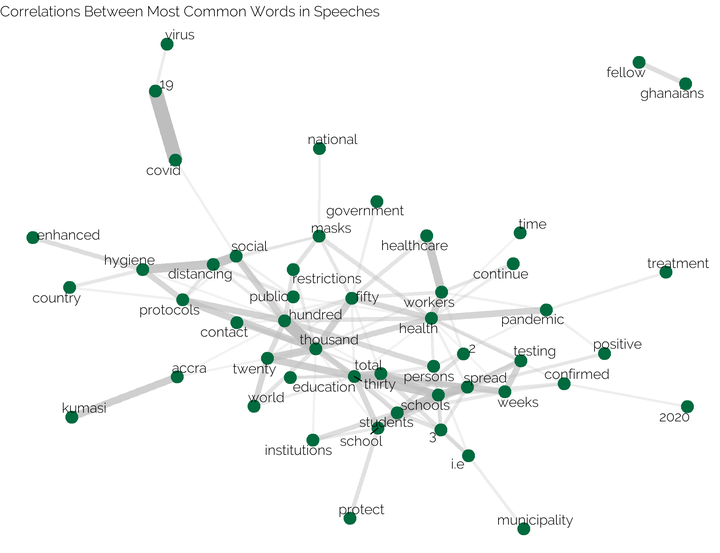
Using the methods described in this chapter, We can also calculate the correlation between different words. Using the phi ($\phi$) coefficient, we can calculate how often words appear together relative to how often they appear separately. To define what ‘together’ means I need to subset the text in different sections. I have decided to do that by dividing the text in sections of 3 sentences each. This is a bit arbitrary, but considering the length of the speeches I do think this works well.
The Tidytext book does a good job explaining this phi ($\phi$) coefficient correlation:
“The focus of the phi coefficient is how much more likely it is that either both word X and Y appear, or neither do, than that one appears without the other. Consider the following table:"
| Has word Y | No word Y | Total | |
|---|---|---|---|
| Has word X | $n_{11}$ | $n_{00}$ | $n_{1\cdot}$ |
| No word X | $n_{01}$ | $n_{00}$ | $n_{0\cdot}$ |
| Total | $n_{\cdot1}$ | $n_{\cdot0}$ | $n$ |
*“For example, that $n_{11}$ represents the number of [sections] where both word X and word Y appear, $n_{00}$ the number where neither appears, and $n_{10}$ and $n_{01}$ the cases where one appears without the other. In terms of this table, the phi coefficient is:"*
$$ \phi = \frac{n_{11}n_{00} - n_{10}n_{01}}{\sqrt{n_{1\cdot} n_{0\cdot} n_{\cdot0} n_{\cdot1}}} $$
To actually calculate this correlation coefficient, I make use of the pairwise_cor() function of the widyr package. I then use ggplot2 with the ggraph extension to create a graph visualization of these correlations. To get the actual input of the plotting function I use the graph_from_data_frame() function from the igraph package.
covid_speeches %>%
  # split text into sentences
  unnest_tokens(sentence, text,
                token = "sentences",
                drop  = T,
                to_lower = F) %>%
  # create different sections (per speech) of 3 sentences
  group_by(title) %>%
  mutate(section = (row_number() %/% 3) + 1) %>%
  ungroup() %>%
  # split text into actual tokens
  unnest_tokens(word, sentence) %>%
  # filter out stop words
  filter(!word %in% stop_words$word) %>%
  group_by(word) %>%
  # omit words that are uncommon
  filter(n() >= 22) %>%
  # calculate correlations
  pairwise_cor(word, section, sort = TRUE) %>%
  # omit combinations with a low correlation
  # otherwise the plot clutters
  filter(correlation > .5) %>%
  # create a graph data frame  using igraph
  graph_from_data_frame() %>%
  # create graph visualization
  ggraph(layout = "fr") + #, algorithm = 'kk') +
  # beautify plot a bit
  geom_edge_link(aes(edge_alpha = correlation, edge_width = correlation), edge_colour = "grey", show.legend = FALSE) +
  # green colour of the Ghanaian flag
  geom_node_point(color = "#006B3F", size = 5) +
  geom_node_text(aes(label = name), repel = TRUE, size = 10, family = "Raleway") +
  theme_void() +
  labs(title = "Correlations Between Most Common Words in Speeches") +
  theme(plot.title  = element_text(family = "Raleway", size =30))
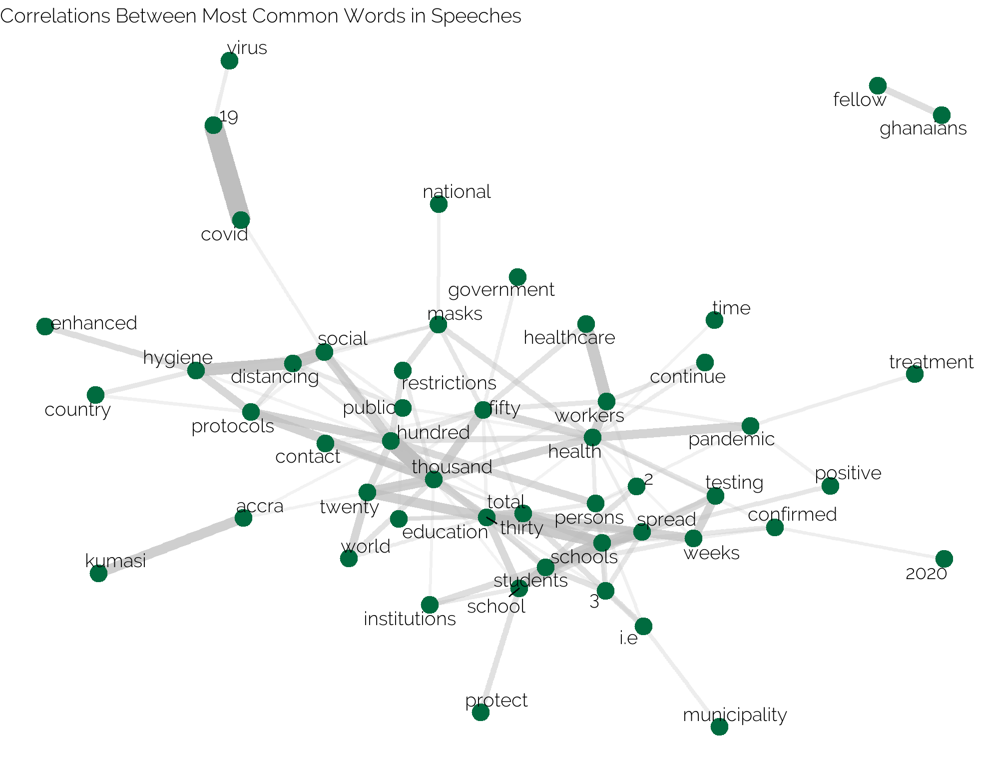
I think this is quite an insightful visualization, that shows which words are commonly used together.
Sentiment analysis.
Now I have inspected the data and determined that it looks good to me, it is time to do the actual sentiment analysis. The most important part of doing a sentiment analysis is getting a lexicon (dictionary) with words with corresponding sentiments. There are many of such dictionaries available, some of which are free to use and others that require a license. I recommend this, this, or this page if you are interested in reading a bit more on available lexicons. I am using the Afinn lexicon. This lexicon scores words on a scale from -5 to -1 for words with a negative sentiment and from 1 to 5 for words with a positive sentiment.
# the latest version of the dictionary can be found here
Afinn <- read.delim("https://raw.githubusercontent.com/fnielsen/afinn/master/afinn/data/AFINN-en-165.txt",
                    header = F) %>%
  as_tibble() %>%
  rename(word = 1,
         sentiment = 2)
This is how this dataset looks:
Afinn %>%
tail() %>%
  kable() %>%
  kable_styling(c("striped", "hover", "condensed"))
| word | sentiment |
|---|---|
| youthful | 2 |
| yucky | -2 |
| yummy | 3 |
| zealot | -2 |
| zealots | -2 |
| zealous | 2 |
Now I can merge these sentiments to the text. After that I can compare the average sentiments of different quintiles of the speeches. Furthermore, I will create some extra statistics, such as the average length (number of sentences) of the speeches
sentence_length <- parsedtxt %>%
  filter(!c(pos %in% c("PUNCT", "SPACE", "NUM"))) %>%
  filter(!token %in% c("%", "&", "-")) %>%
  group_by(speech, sentence_nr ) %>%
  summarise(n_words = n(), .groups = "drop") %>%
  group_by(speech) %>%
  summarise(mean_sentence_length = mean(n_words),
            n_sentences = n()) %>%
  left_join(covid_speeches %>% select(title, date),
            by = c("speech" = "title"))
parsedtxt %>%
  # join sentiments
  left_join(Afinn, by = c("lemma"= "word")) %>%
  group_by(speech,  sentence_nr) %>%
  # if there is no sentiment in the sentence, I make the sentiment 0.
  mutate(sentiment = ifelse(is.na(sentiment), 0, sentiment)) %>%
  # calculate the mean sentiment per sentence
  summarise(sentiment_mean = mean(sentiment, na.rm =T), .groups = "drop") %>%
  group_by(speech) %>%
  # split text into quintiles
  arrange(speech,  sentence_nr) %>%
  mutate(section = ntile( sentence_nr , 5)) %>%
  # calculate the mean sentiment per quintiles
  group_by(speech, section) %>%
  summarise(mean_Sep = mean(sentiment_mean)) %>%
  # spread the results from a long to a wide format
  pivot_wider(values_from  = mean_Sep,
              names_from = section,
              names_prefix = "section_") %>%
  # compare the mean of the first 4 section to the last section
  mutate(diff_sec_sec1_4 = section_5 - mean(c(section_1,section_2, section_3, section_4) )) %>%
  ungroup() %>%
  # add sentence length statistics
  right_join(sentence_length, by = "speech") %>%
  arrange(date) %>%
  # select columns
  select(speech, date, n_sentences, mean_sentence_length, section_1:diff_sec_sec1_4) %>%
  # round values
  mutate(across(where(is.numeric),  ~round(., 4))) %>%
  kable() %>%
  kable_styling(c("striped", "hover", "condensed"))
| speech | date | n_sentences | mean_sentence_length | section_1 | section_2 | section_3 | section_4 | section_5 | diff_sec_sec1_4 |
|---|---|---|---|---|---|---|---|---|---|
| President Akufo-Addo Addresses Nation On Measures Taken By Gov't To Combat The Coronavirus Pandemic | 2020-03-15 | 27 | 23.2222 | 0.0055 | -0.0051 | 0.0112 | 0.0713 | 0.1588 | 0.1381 |
| Address To The Nation By President Akufo-Addo On Updates To Ghana’s Enhanced Response To The Coronavirus Pandemic | 2020-03-27 | 128 | 17.1250 | 0.0567 | 0.0000 | 0.0135 | 0.0148 | 0.1107 | 0.0894 |
| Address To The Nation By President Akufo-Addo On Updates To Ghana’s Enhanced Response To The Coronavirus Pandemic | 2020-04-05 | 108 | 25.8981 | 0.0681 | 0.0111 | 0.0323 | 0.0037 | 0.0497 | 0.0208 |
| President Akufo-Addo On Updates To Ghana’s Enhanced Response To COVID-19 | 2020-04-09 | 68 | 21.8235 | 0.0297 | 0.0518 | -0.0071 | 0.1752 | 0.1436 | 0.0812 |
| President Akufo-Addo Provides Update On Measures Taken Against Spread of COVID-19 | 2020-04-26 | 110 | 24.0545 | -0.0046 | 0.0336 | -0.0473 | 0.0435 | 0.0447 | 0.0384 |
| President Akufo-Addo Provides Update On Ghana’s Enhanced Response To COVID-19 | 2020-05-10 | 80 | 28.4000 | 0.0305 | -0.0105 | -0.0144 | 0.0541 | 0.0936 | 0.0787 |
| Update No.10: Measures Taken To Combat Spread Of Coronavirus | 2020-05-31 | 94 | 27.1915 | 0.0265 | 0.0113 | 0.0015 | 0.0351 | 0.0922 | 0.0736 |
| Update No.11: Measures Taken To Combat Spread Of Coronavirus | 2020-06-14 | 86 | 26.1279 | 0.0460 | 0.0284 | 0.0471 | -0.0502 | 0.0615 | 0.0437 |
| Update No 12: Measures Taken To Combat Spread Of Coronavirus | 2020-06-21 | 91 | 24.4945 | 0.0592 | -0.0010 | -0.0122 | -0.0186 | 0.0471 | 0.0403 |
| Update No 13: Measures Taken To Combat Spread Of Coronavirus | 2020-06-28 | 66 | 25.1061 | 0.0426 | 0.0130 | -0.0510 | 0.0219 | 0.0577 | 0.0510 |
| Update No 14: Measures Taken To Combat Spread Of Coronavirus | 2020-07-26 | 112 | 24.8036 | 0.0676 | 0.0422 | 0.0035 | 0.0218 | 0.0253 | -0.0085 |
With only one exception, the latest speech by the president, all speeches had a final quintile that is more positive than the first 80% of the speech.
The same pattern can be observed if I plot the average sentiment per sentence compared to the sentence number. In this plotting I made the decision to only plot the a smoothed line through the different points, instead of the points themselves (that would be too cluttered). I use a Loess function (a generalized Savitzky–Golay filter with variable window size) to do the smoothing. My main difficulty with the plotting was that I wanted to create a function that shows the actual text of a sentence with positive words highlighted green and negative words highlighted in different shades of red.
colfunc_red <- colorRampPalette(c("#ff5252","#a70000"))
colfunc_green <- colorRampPalette(c("#A3D12D","#086D44"))


# get text data and use html tags to colour words green or red
text <- parsedtxt %>%
  left_join(Afinn, by = c("lemma"= "word")) %>%
  mutate(sentiment = ifelse(is.na(sentiment), 0, sentiment)) %>%
  mutate(token_colour = ifelse(sentiment < 0,
                         paste0('<span style="color:',
                                colfunc_red(abs(min(sentiment)))[abs(sentiment)],
                                ';"><b>',  token,'</b></span>'),
                         ifelse(sentiment > 0,
                                paste0('<span style="color:',
                                       colfunc_green(abs(max(sentiment)))[abs(sentiment)],
                                       ';"><b>', token,'</b></span>'),
                                token))) %>%
  mutate(nchar_token = nchar(token)) %>%
  group_by(speech, sentence_nr) %>%
  arrange(sentence_nr) %>%
  # I also want to break up long sentences
  mutate(nchar_token_cum = cumsum(nchar_token)) %>%
  mutate(split = which.min(abs(nchar_token_cum - 60))) %>%
  mutate(split2 = which.min(abs(nchar_token_cum - 120))) %>%
  mutate(split3 = which.min(abs(nchar_token_cum - 180))) %>%
  mutate(split4 = which.min(abs(nchar_token_cum - 240))) %>%
  mutate(token_colour = ifelse(token_id == split & max(nchar_token_cum) >=120 ,
                               paste0(token_colour, "<br>"),
                               token_colour)) %>%
  mutate(token_colour = ifelse(token_id == split2 & max(nchar_token_cum) >=120 ,
                               paste0(token_colour, "<br>"),
                               token_colour)) %>%
  mutate(token_colour = ifelse(token_id == split3 & max(nchar_token_cum) >=180 ,
                               paste0(token_colour, "<br>"),
                               token_colour)) %>%
  mutate(token_colour = ifelse(token_id == split4 & max(nchar_token_cum) >=240 ,
                               paste0(token_colour, "<br>"),
                               token_colour)) %>%
  # Now I have added the colours to the words I can collapse them back into sentences
  summarise(collapsed_sentence = paste0(token_colour, collapse=" ")) %>%
  mutate(# delete space before comma
         collapsed_sentence = gsub(" ,", ",", collapsed_sentence),
         # delete space before full stop
         collapsed_sentence = gsub(" \\.", ".", collapsed_sentence),
         # delete space before exclamation point
         collapsed_sentence = gsub(" !", "!", collapsed_sentence),
         # delete space around hyphens
         collapsed_sentence = gsub(" - ", "-", collapsed_sentence),
         # delete space around brackets
         collapsed_sentence = gsub("\\( ", "(", collapsed_sentence),
         # delete space around brackets
         collapsed_sentence = gsub(" \\)", ")", collapsed_sentence)) %>%
  ungroup() %>%
  # Now I just add the dates to the speeches
  left_join(sentence_length %>% select(speech, date), by = "speech")
After formatting the words into sentences, I also need to calculate the average sentiment per sentence and then smooth the data grouped by speech using the broom package. After that I add the dates to the speech labels and order the speeches in chronological order.
dat <- parsedtxt %>%
   filter(!c(pos %in% c("PUNCT", "SPACE", "NUM"))) %>%
  filter(!token %in% c("%", "&", "-"))  %>%
  left_join(Afinn, by = c("lemma"= "word")) %>%
  group_by(speech,  sentence_nr) %>%
  mutate(sentiment = ifelse(is.na(sentiment), 0, sentiment)) %>%
  summarise(sentiment_mean = mean(sentiment, na.rm = T), .groups = "drop") %>%
  group_by(speech) %>%
  group_by(speech,  sentence_nr) %>%
  nest(data = -speech) %>%
  # use combination of map and augment to get the fitted values of the Loess regression
  mutate(
    fit = map(data, ~ loess(sentiment_mean ~ sentence_nr,
                            data = .x,
                            span = 0.5)),
    augmented = map(fit, augment)) %>%
  # unnest the datasets per speech into one big dataset
  unnest(augmented)  %>%
  select(-data, - fit, - .resid) %>%
  ungroup()

# combine the text and speech data
dat2 <- left_join(dat, text, by = c("sentence_nr", "speech" )) %>%
  mutate(speech = paste0(speech, " (", date, ")")) %>%
  # order speeches
  mutate(speech = fct_reorder(speech, date))
I want to colour the lines that represent the different speeches in different in different colours. So I create a colour palette that is based on the colours of the Ghanaian coat of arms (https://www.schemecolor.com/ghana-coat-of-arms-colors.php).
# create a color palette from the colours of the Ghanaian coat of arms
colfunc <- colorRampPalette(c("#CE1126","#FCD116","#006B3F", "#0193DD", "#000000"))
# now all of this can be combined into a plotly plot
fig3 <- plot_ly(data = dat2,
        type = 'scatter',
        mode = "lines",
        color = ~speech,
        sort = FALSE,
        colors = colfunc(11)) %>%
  add_trace(
    y = ~.fitted,
    x = ~sentence_nr,
    text = ~collapsed_sentence,
    hoverinfo = 'text',
    hoverlabel = list(  bgcolor = "white",
                        opacity = 0.5,
                        size = 7,
                        font= list(family = 'Raleway'),
                        align = "left",
                        line = list(
                          opacity = 0.9,
                          width = 3)),
    showlegend = T)  %>%
  layout(title = list(text = "<b>Sentiment of COVID-19 Speeches by the President of Ghana</b><br><sup>Speeches vary in length, but all end on a positive note.</sup>",
                      x =0.05,
                      xanchor = "left",
                      automargin = TRUE),
         font = list(color = '#706f6f',
                     family = 'Raleway',
                     size = 14),
         xaxis = list(title = "Sentence number",
                      showspikes = TRUE,
                      spikemode  = 'toaxis',
                      spikesnap = 'data',
                      showline = TRUE,
                      showgrid = FALSE,
                      showticklabels = TRUE,
                      linecolor = '#706f6f',
                      linewidth = 2,
                      autotick = TRUE,
                      ticks = 'outside',
                      tickcolor = '#706f6f',
                      tickwidth = 2,
                      ticklen = 5,
                      tickfont = list(family = 'Raleway',
                                      size = 12,
                                      color = '#706f6f')),
         yaxis = list(title = "Average sentence sentiment (smoothed)",
                      showline = TRUE,
                      showgrid = FALSE,
                      showticklabels = TRUE,
                      linecolor = '#706f6f',
                      linewidth = 2,
                      autotick = TRUE,
                      ticks = 'outside',
                      tickcolor = '#706f6f',
                      tickwidth = 2,
                      ticklen = 5,
                      tickfont = list(family = 'Raleway',
                                      size = 12,
                                      color = '#706f6f')),
         legend = list(title = list(text = "<b>Speeches</b><br><sup>(double click on a speech to isolate it and hover over lines to see text)</sup>"),
                       x = 0, y = -.8,
                       xanchor = "left"),
         autosize = T,
         margin = list(t = 100),
         showlegend = TRUE) %>%
  add_annotations( x = 1,
                   y = -0.05,
                   xanchor = "left",
                   showarrow = F,
                   align = "left",
                   text=  '<span style="color:#a70000;"><b>Negative values signify<br>negative sentiment</b></span>') %>%
  add_annotations( x = 1,
                   y = 0.3,
                   xanchor = "left",
                   showarrow = F,
                   align = "left",
                   text=  '<span style="color:#A3D12D;"><b>Positive values signify<br>positive sentiment</b></span>') %>%
  config(displayModeBar = FALSE)

fig3
Limitations
Sentiment analysis is a bit controversial, so I think it is important to note some limitations of the analyses presented in this blog:
- Most importantly this analysis did only take into consideration the English language parts of the speeches. In some of the speeches the president did use some Twi. As of now I do not think any Twi languages dictionaries exist.
- I have not make use of any negators in my analysis. So the sentence “I am not happy," might have a positive sentiment, because I did not control for the “not” prior to “happy."
- You can argue about the validity of these sentiment lexicons. For example the word “fight” has a negative sentiment in this lexicon, but maybe you consider a fight (against COVID-19) a positive thing. This is especially true for the word “positive” in the context of COVID-19. The term “positive tests” is used frequently, but is not necessarily a positive thing.
Valuable Information and Tutorials
These are some further valuable sources on these types of analysis:
- Harvesting the web with rvest
- Web Scraping in R: rvest Tutorial
- Interactive web-based data visualization with R, plotly, and shiny
- broom and dplyr
- Text Mining with R
- Spacy 101
All of these sources helped me write this post.
Ghana Data Stuff
This website is my hobby project to showcase some of the project I am working one, when I am not working on the official statistics at the Ghana Statistical Service.